LaMa and RTMB
LaMa_and_RTMB.RmdBefore diving into this vignette, we recommend reading the vignettes Introduction to LaMa, Inhomogeneous HMMs and Periodic HMMs.
The recently introduced R package RTMB
conveniently allows for automatic differentiation for non-standard
statistical models written in plain R code. This enables
the estimation of very complicated models, potentially with complex
random effect structures. The process feels like magic because you have
access to analytic gradients – drastically increasing accuracy
and speed – without doing any calculations!
LaMa is now also fully compatible with AD provided by
RTMB. Hence, estimation of latent Markov models is now
faster and more convenient, while model specification is very smooth and
less prone to errors – which at the current state tend to happen when
one is not experienced with RTMB.
Here we demonstrate how to use LaMa and
RTMB to fit hidden Markov models and their extensions. We
start by loading the LaMa package, which automatically
loads RTMB as well.
For the purpose of this vignette, we will analyse the
trex data set contained in the package. It contains hourly
step lengths of a Tyrannosaurus rex, living 66 million years ago, and we
aim to understand its behavioural process using HMMs.
head(trex, 5)
#>   tod      step     angle state
#> 1   9 0.3252437        NA     1
#> 2  10 0.2458265  2.234562     1
#> 3  11 0.2173252 -2.262418     1
#> 4  12 0.5114665 -2.958732     1
#> 5  13 0.3828494  1.811840     1
Basic workflow
The workflow with RTMB is basically always the same. We
need to
- define the negative log-likelihood function,
- create an automatically differentiable objective function from it and
- fit the model by numerical minimisation of the latter.
RTMB also provides many functions that make this process
very convenient.
Simple HMM
We start by fitting a super simple stationary HMM with
state-dependent gamma distributions for the step lengths and von Mises
distributions for the turning angles. As a first step, we define the
initial parameter list par and a dat list that
contains the data and potential hyperparameters – here N, the number of hidden states. The names
par and dat are of course arbitrary.
par = list(
  logmu = log(c(0.3, 1)),      # initial means for step length (log-transformed)
  logsigma = log(c(0.2, 0.7)), # initial sds for step length (log-transformed)
  logkappa = log(c(0.2, 0.7)), # initial concentration for turning angle (log-transformed)
  eta = rep(-2, 2)             # initial t.p.m. parameters (on logit scale)
  )

dat = list(
  step = trex$step,   # hourly step lengths
  angle = trex$angle, # hourly turning angles
  N = 2
  )
As par is a named list of initial parameter values,
accessing the parameters later on is much more convenient than indexing.
You can also use a parameter vector with RTMB, but using a
named list makes our life so much easier.
We can now define the negative log-likelihood function in a similar fashion to basic numerical ML
nll = function(par) {
  getAll(par, dat) # makes everything contained available without $
  Gamma = tpm(eta) # computes transition probability matrix from unconstrained eta
  delta = stationary(Gamma) # computes stationary distribution
  # exponentiating because all parameters strictly positive
  mu = exp(logmu)
  sigma = exp(logsigma)
  kappa = exp(logkappa)
  # reporting statements for later use
  REPORT(mu); ADREPORT(mu)
  REPORT(sigma); ADREPORT(sigma)
  REPORT(kappa); ADREPORT(kappa)
  # calculating all state-dependent densities
  allprobs = matrix(1, nrow = length(step), ncol = N)
  ind = which(!is.na(step) & !is.na(angle)) # only for non-NA obs.
  for(j in 1:N){
    allprobs[ind,j] = dgamma2(step[ind],mu[j],sigma[j])*dvm(angle[ind],0,kappa[j])
  }
  -forward(delta, Gamma, allprobs) # simple forward algorithm
}
but a few points should be made here:
- Most prominently, the negative log-likelihood is a function of the
parameters to be estimated only while data and other parameters
are not passed as an argument at this stage. This is something to get
used to (I know), but just the way
RTMBworks. - The
getAll()function is very useful and you should use it in the first line to unpack both theparand thedatlist, making all elements available without the$operator. At this stage,nlljust takes the dat object from the global environment. - Parameter transformations are of course still necessary, i.e. all
parameters in
parshould be unconstrained. - You might wonder how on earth
RTMBcan calculate the gradient of parameters in distributions like the gamma or von Mises distribution. The answer is: It can’t but provides its own version of all standard distributions likednorm(),dbinom(), etc. In this case bothdgamma2()anddvm()come fromLaMaas these are non-standard, but under the hood build onRTMBfunctions (dgamma2()is actually just a convenience function that reparametrises the gamma distribution in terms of mean and standard deviation). - Actually, most of the standard functions (e.g.
sum()), operators (e.g.%*%) and methods (e.g.matrix) are “overwritten” when called insideMakeADFun()but you typically don’t notice that and should not care. - the
REPORT()function offered byRTMBis really convenient as any quantities calculated in the likelihood function (for which you have written the code anyway), if reported, will be available after optimisation, while the report statements are ignored during optimisation. So no annoying backtransformations anymore, woohoo! - for simple parameter transformations,
ADREPORT()is also great, because it calculates standard deviations forADREPORT()ed quantities, based on the delta method. Just note that the delta method is not advisable for complex non-linear and multivariate transformations.
Having defined the negative log-likelihood, we can now create the
automatically differentiable objective function and fit the model. This
needs a little explanation: At this point, RTMB takes the
negative log-likelihood function and generates its own (very fast)
version of it, including a gradient. MakeADFun() now also
grabs whatever is saved as dat in the global environment
and bakes it into the objective function. Therefore, changes to
dat after this point will have no effect on the
optimisation result. We set silent = TRUE to suppress
printing of the optimisation process.
obj = MakeADFun(nll, par, silent = TRUE) # creating the objective functionLet’s check out obj:
names(obj)
#>  [1] "par"          "fn"           "gr"           "he"           "hessian"
#>  [6] "method"       "retape"       "env"          "report"       "simulate"
#> [11] "force.update"
It contains the initial parameter par (now transformed
to a named vector), the objective function fn (which in
this case just evaluates nll but faster), its gradient
gr and Hessian he.
If we now call these functions without any argument, we get the corresponding values at the initial parameter vector.
obj$par
#>      logmu      logmu   logsigma   logsigma   logkappa   logkappa        eta
#> -1.2039728  0.0000000 -1.6094379 -0.3566749 -1.6094379 -0.3566749 -2.0000000
#>        eta
#> -2.0000000
obj$fn()
#> [1] 33293.84
obj$gr()
#>          [,1]      [,2]     [,3]      [,4]     [,5]      [,6]     [,7]
#> [1,] 573.7198 -2467.274 95.35893 -12045.97 55.92507 -807.9504 134.0732
#>           [,8]
#> [1,] -181.2148
We are now ready to optimise the objective function. The optimisation
routine nlminb() is very robust and conveniently allows us
to provide a gradient function. Alternatively, you can also use
optim() or any other optimiser you like that allows you to
pass a gradient function.
Indeed, we do not provide the Hessian to nlminb()
because, while evaluating the Hessian is very fast with
RTMB, optimisation is still much faster if we use a
quasi-Newton algorithm that approximates the current Hessian based on
previous gradient evaluations, compared to using full
Newton-Raphson.
opt = nlminb(obj$par, obj$fn, obj$gr) # optimizationWe can check out the estimated parameter and function value by
opt$par
#>      logmu      logmu   logsigma   logsigma   logkappa   logkappa        eta
#> -1.1916144  0.9182131 -1.5995349  0.3999258 -2.2872716  0.4019563 -1.6621910
#>        eta
#> -1.5735921
opt$objective
#> [1] 27248.59
Note that the naming here is determined by nlminb(). If
you use a different optimiser, these may be called differently.
Much nicer however, is that obj (yes obj
not opt) is automatically updated after the optimisation.
Note that calling obj$gr() after optimisation now gives the
gradient at the optimum, while obj$fn() still gives the
objective at the starting value and obj$par is not updated
but still the initial parameter vector (kind of confusing).
To get our estimated parameters on their natural scale, we don’t have to do the backtransformation manually. We can just run the reporting:
mod = obj$report() # runs the reporting from the negative log-likelihood once
(delta = mod$delta)
#>       S1       S2
#> 0.481525 0.518475
(Gamma = mod$Gamma)
#>           S1        S2
#> S1 0.8282951 0.1717049
#> S2 0.1594681 0.8405319
(mu = mod$mu)
#> [1] 0.3037305 2.5048106
(sigma = mod$sigma)
#> [1] 0.2019904 1.4917139
(kappa = mod$kappa)
#> [1] 0.1015431 1.4947460
which works because of the REPORT() statements in the
likelihood function. Note that delta, Gamma
and allprobs are always reported by default when using
forward() which is very useful for e.g. state decoding with
viterbi(), because many downstream LaMa
functions take these arguments as inputs. Functions of the
viterbi and stateprobs family can also take
the reported list object as an input. As the state-dependent parameters
depend on the specific model formulation, these need to be reported
manually by the user specifying the negative log-likelihood. Having all
the parameters, we can plot the decoded time series
# manually
mod$states = viterbi(mod$delta, mod$Gamma, mod$allprobs)

# or simpler
mod$states = viterbi(mod = mod)

# defining color vector
color = c("orange", "deepskyblue")

plot(trex$step[1:200], type = "h", xlab = "time", ylab = "step length",
     col = color[mod$states[1:200]], bty = "n")
legend("topright", col = color, lwd = 1, legend = c("state 1", "state 2"), bty = "n")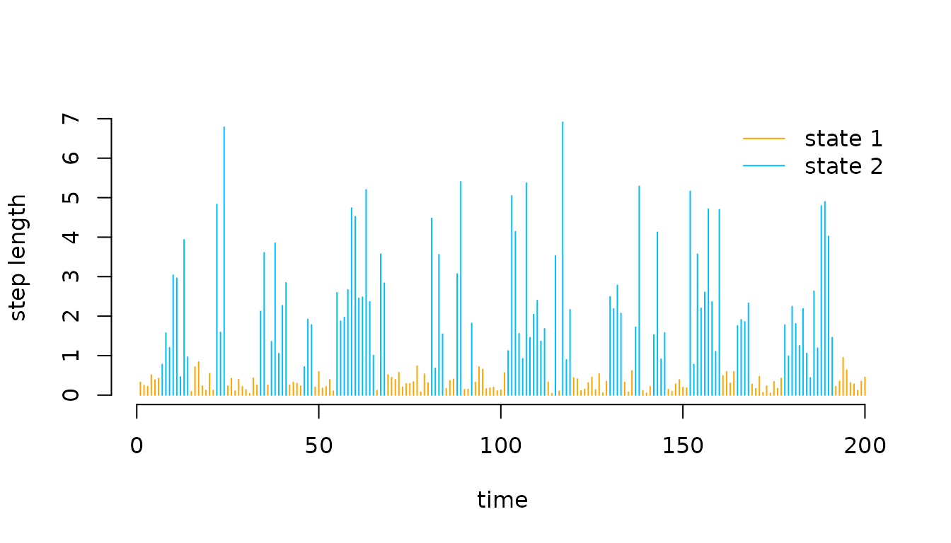
or the estimated state-dependent distributions.
oldpar = par(mfrow = c(1,2))
hist(trex$step, prob = TRUE, breaks = 40,
     bor = "white", main = "", xlab = "step length")
for(j in 1:2) curve(delta[j] * dgamma2(x, mu[j], sigma[j]),
                    lwd = 2, add = T, col = color[j])
curve(delta[1]*dgamma2(x, mu[1], sigma[1]) + delta[2]*dgamma2(x, mu[2], sigma[2]),
      lwd = 2, lty = 2, add = T)
legend("top", lwd = 2, col = color, legend = c("state 1", "state 2"), bty = "n")

hist(trex$angle, prob = TRUE, breaks = 40,
     bor = "white", main = "", xlab = "turning angle")
for(j in 1:2) curve(delta[j] * dvm(x, 0, kappa[j]),
                    lwd = 2, add = T, col = color[j])
curve(delta[1]*dvm(x, 0, kappa[1]) + delta[2]*dvm(x, 0, kappa[2]),
      lwd = 2, lty = 2, add = T)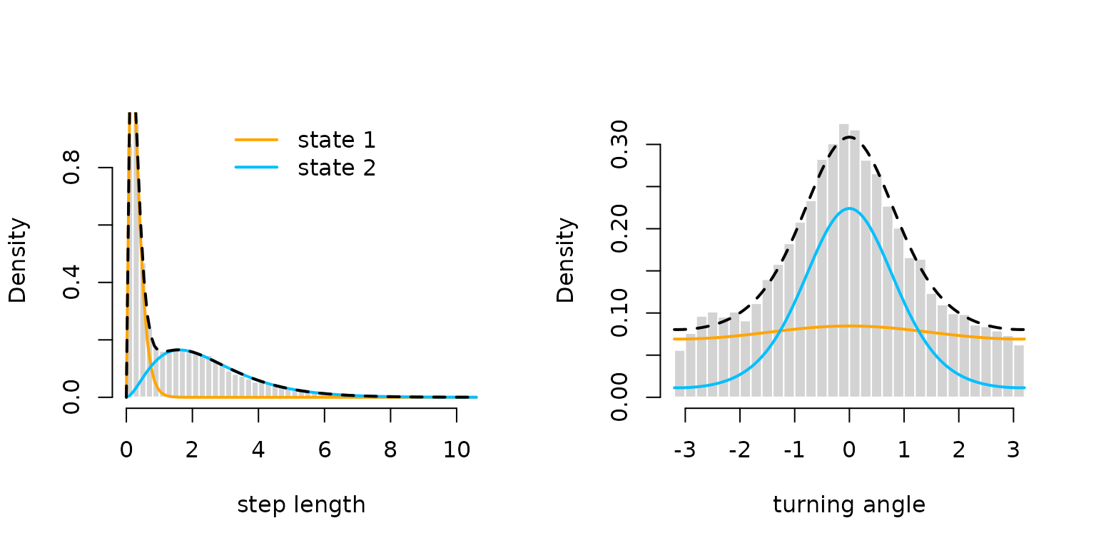
par(oldpar) # resetting to defaultMoreover, we can also use the sdreport() function to
directly give us standard errors for our unconstrained parameters and
everything we ADREPORT()ed.
sdr = sdreport(obj)We can then get an overview of the estimated parameters and
ADREPORT()ed quantities as well as their standard errors
by
summary(sdr)
#>            Estimate  Std. Error
#> logmu    -1.1916144 0.011067932
#> logmu     0.9182131 0.008875692
#> logsigma -1.5995349 0.016232361
#> logsigma  0.3999258 0.013272894
#> logkappa -2.2872716 0.207126331
#> logkappa  0.4019563 0.019299344
#> eta      -1.6621910 0.041754277
#> eta      -1.5735921 0.040795512
#> mu        0.3037305 0.003361669
#> mu        2.5048106 0.022231928
#> sigma     0.2019904 0.003278782
#> sigma     1.4917139 0.019799361
#> kappa     0.1015431 0.021032256
#> kappa     1.4947460 0.028847617
To get the estimated parameters or their standard errors in list format, type
# estimated parameter in list format
as.list(sdr, "Estimate")
# parameter standard errors in list format
as.list(sdr, "Std")
and to get the estimates and standard errors for
ADREPORT()ed quantities in list format, type
# adreported parameters as list
as.list(sdr, "Estimate", report = TRUE)
# their standard errors
as.list(sdr, "Std", report = TRUE)
Lastly, the automatic reporting with LaMa and
RTMB together makes calculating pseudo-residuals really
convenient:
pres_step = pseudo_res(trex$step, "gamma2", list(mean = mu, sd = sigma), mod = mod)
plot(pres_step, hist = TRUE)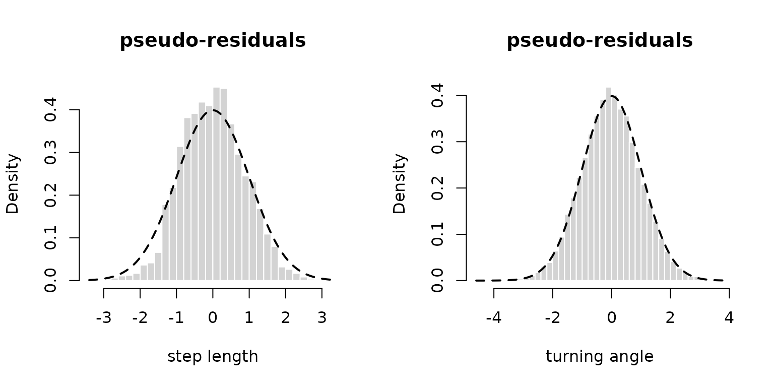
pres_angle = pseudo_res(trex$angle, "vm", list(mu = 0, kappa = kappa), mod = mod)
plot(pres_angle, hist = TRUE)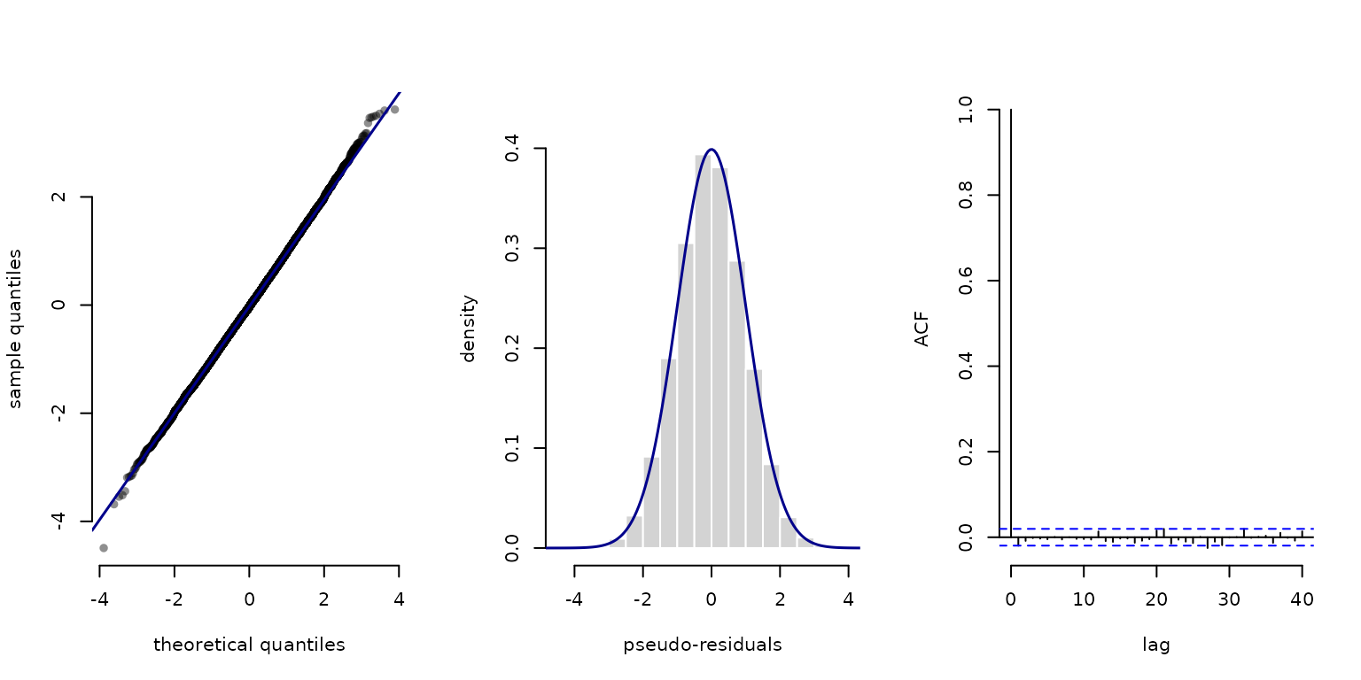
Covariate effects
We can now generalise the previous model to include covariate effects. In our example, we might be interested how the T-rex’s behaviour varies with the time of day. Hence, we add diel variation to the state process. For example, we can model the transition probabilities as a function of the time of day using a trigonometric basis expansion to ensure diurnal continuity. The transition probabilities are given by \text{logit}(\gamma_{ij}^{(t)}) = \beta_0^{(ij)} + \beta_1^{(ij)} \sin \bigl(\frac{2 \pi t}{24}\bigr) + \beta_2^{(ij)} \cos \bigl(\frac{2 \pi t}{24}\bigr) + \beta_3^{(ij)} \sin \bigl(\frac{2 \pi t}{12}\bigr) + \beta_4^{(ij)} \cos \bigl(\frac{2 \pi t}{12}\bigr), where t is the time of day.
To practically achieve this, we compute the trigonometric basis
design matrix Z corresponding to above predictor and add
the time of day to the dat list for indexing inside the
likelihood function. The LaMa function
cosinor() does this very conveniently. We can either call
it directly to build the design matrix, or use it in a
formula passed to make_matrices(). The latter
is preferable when dealing with more complicated models. Note that the
first option does not include an intercept column, while the second
does. When used with tpm_g() this does not matter as it
automatically checks if an intercept column is included.
Z = cosinor(1:24, period = c(24, 12))

modmat = make_matrices(~ cosinor(tod, period = c(24, 12)),
                       data = data.frame(tod = 1:24))
Z = modmat$Z

# only compute the 24 unique values and index later for entire time series
dat$Z = Z # adding design matrix to dat
dat$tod = trex$tod # adding time of day to dat for indexing
We also need to change the parameter list par to include
the regression parameters for the time of day. The regression parameters
for the state process will typically have the form of a N (N-1) \times p+1 matrix, where N is the number of states and p is the number of regressors – this format
is also expected by tpm_g() which computes the array of
transition matrices based on the design and parameter matrix. Another
lovely convenience that RTMB allows for is that, in our
parameter list, we can have matrices, making reshaping of vectors to
matrices inside the likelihood function unnecessary.
par = list(logmu = log(c(0.3, 1)),
           logsigma = log(c(0.2, 0.7)),
           logkappa = log(c(0.2, 0.7)),
           beta = matrix(c(rep(-2, 2),
                           rep(0, 2*4)), nrow = 2)) # 2 times 4+1 matrix
# replacing eta with regression parameter matrix, initializing slopes at zero
We can now define a more general likelihood function with the main
difference being the use of tpm_g() instead of
tpm() and the inclusion of the time of day in the
transition matrix calculation. This leads to us using
stationary_p() instead of stationary() to
calculate the initial distribution and forward_g() instead
of forward() to calculate the log-likelihood.
nll2 = function(par) {
  getAll(par, dat) # makes everything contained available without $
  Gamma = tpm_g(Z, beta) # covariate-dependent tpms (in this case only 24 unique)
  # tpm_g() automatically checks if intercept column is included
  ADREPORT(Gamma) # adreporting
  Delta = stationary_p(Gamma) # all periodically stationary distributions
  ADREPORT(Delta)
  delta = Delta[tod[1],] # initial periodically stationary distribution
  # exponentiating because all parameters strictly positive
  mu = exp(logmu); REPORT(mu)
  sigma = exp(logsigma); REPORT(sigma)
  kappa = exp(logkappa); REPORT(kappa)
  # calculating all state-dependent densities
  allprobs = matrix(1, nrow = length(step), ncol = N)
  ind = which(!is.na(step) & !is.na(angle)) # only for non-NA obs.
  for(j in 1:N){
    allprobs[ind,j] = dgamma2(step[ind],mu[j],sigma[j])*dvm(angle[ind],0,kappa[j])
  }
  -forward_g(delta, Gamma[,,tod], allprobs) # indexing 24 unique tpms by tod in data
}
Having done this, the model fit is then essentially the same:
obj2 = MakeADFun(nll2, par, silent = TRUE) # creating the objective function
opt2 = nlminb(obj2$par, obj2$fn, obj2$gr) # optimisation
and we can look at the reported results. In this case, for simplicity
I get standard errors for Gamma with the delta method
while, in general, this is not advisable.
mod2 = obj2$report()

sdr = sdreport(obj2)
Gamma = as.list(sdr, "Estimate", report = TRUE)$Gamma
Gammasd = as.list(sdr, "Std", report = TRUE)$Gamma

Delta = as.list(sdr, "Estimate", report = TRUE)$Delta
Deltasd = as.list(sdr, "Std", report = TRUE)$Delta

tod_seq = seq(0, 24, length = 200) # sequence for plotting
Z_pred = trigBasisExp(tod_seq, degree = 2) # design matrix for prediction

Gamma_plot = tpm_g(Z_pred, mod2$beta) # interpolating transition probs

plot(tod_seq, Gamma_plot[1,2,], type = "l", lwd = 2, ylim = c(0,1),
     xlab = "time of day", ylab = "transition probability", bty = "n")
segments(x0 = 1:24, y0 = Gamma[1,2,]-1.96*Gammasd[1,2,],
         y1 = Gamma[1,2,]+1.96*Gammasd[1,2,])
segments(x0 = 1:24, y0 = Gamma[2,1,]-1.96*Gammasd[2,1,],
         y1 = Gamma[2,1,]+1.96*Gammasd[2,1,])
lines(tod_seq, Gamma_plot[2,1,], lwd = 2, lty = 3)
legend("topleft", lwd = 2, lty = c(1,3), bty = "n",
       legend = c(expression(gamma[12]^(t)), expression(gamma[21]^(t))))
plot(Delta[,2], type = "b", lwd = 2, xlab = "time of day", ylab = "Pr(active)",
     col = "deepskyblue", bty = "n", xaxt = "n")
segments(x0 = 1:24, y0 = Delta[,2]-1.96*Deltasd[,2], lwd = 2,
         y1 = Delta[,2]+1.96*Deltasd[,2], col = "deepskyblue")
axis(1, at = seq(0,24,by=4), labels = seq(0,24,by=4))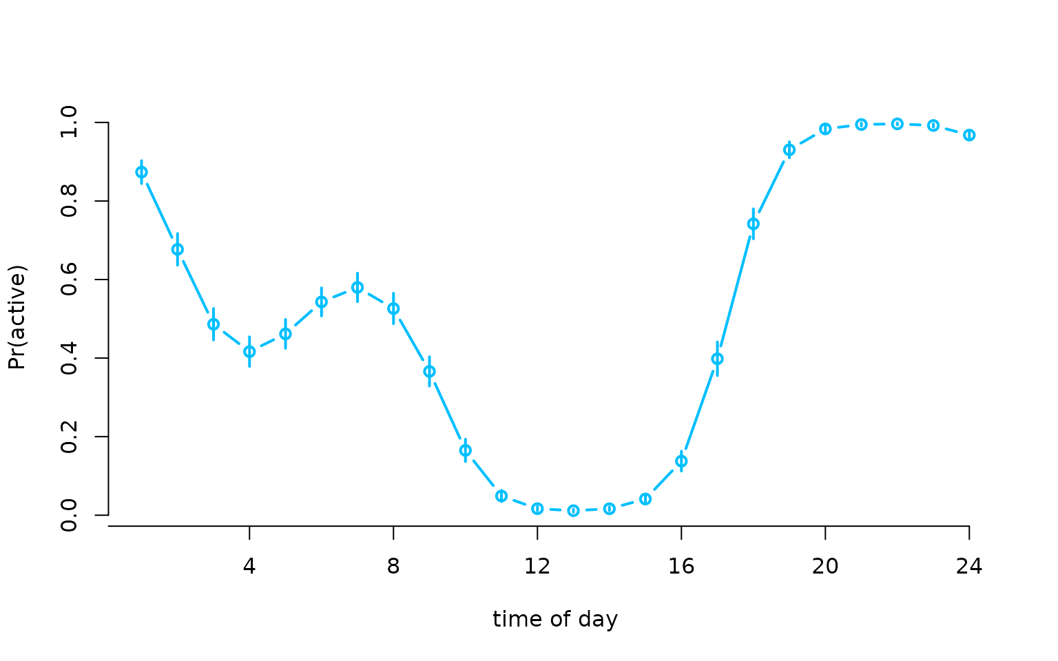
RTMB tips and issues
Tips
When using the forward algorithm, it is usually a good idea to run:
RTMB::TapeConfig(matmul = "plain")This changes how RTMB internally represents matrix
multiplications and can speed up the forward algorithm considerably.
If you want to use non-standard probability distributions, check-out
the R package RTMBdist
which provides a library of AD-compatible distributions
that can be used inside likelihood functions.
Common issues
There are some problems with RTMB one has to keep in
mind. They can be a bit annoying, but in my opinion the benefits of
automatic differentiation far outweigh the drawbacks. I list the main
ones I have encountered here, but please tell me if you encounter more,
such that they can be added.
A typical issue with RTMB is that some operators might
need to be overloaded to allow for automatic differentiation which
cannot be done by default. In typical model setups LaMa
functions do this themselves, but if you go a very individualistic route
and get an error like
stop("Invalid argument to 'advector' (lost class attribute?)")you might have to overload the operator yourself. To do this put
"[<-" <- ADoverload("[<-")as the first line of your likelihood function. If the error still prevails also add
"c" <- ADoverload("c")
"diag<-" <- ADoverload("diag<-")
which should hopefully fix the error.
Another common problem occurs when initiating objects with
NA values and then trying to fill them with
numeric values. This is because NA is logical
which screws up the automatic differentiation due to the mismatching
types. To avoid this, always initiate with numeric or
NaN values. For example, don’t do
but rather
to avoid the error.
If you create and array and fill with something parameter-dependent, you should also do:
This makes sure that X is an AD object from the
beginning and classes are compatible.
Wrapping things in AD() is generally a good idea to fix
the above error, as it does not introduce considerable overhead when not
necessary.
Importantly, you cannot use if or max/
min statements on the parameter itself as
these are not differentiable. If you do so, RTMB will fail
and probably does not produce a helpful error message. The problem here
results from RTMB building the tape (computational
graph) of the function at the initial parameter value. When you have
if statements, the resulting gradient will be different
from the one at a different parameter value. Often, you can remedy this
behaviour by exploiting the fact that abs() is
differentiable (in code). For example, you can create the differentiable
max alternative:
max2 = function(x,y){
  (x + y + abs(x - y)) / 2
}
So you might be able to solve such problems by finding a clever
alternative. If the if statement does not involve the
parameter, it will typically be fine because it does not change during
the optimisation.
Furthermore, there are some unfortunate side effects of R’s ‘byte compiler’ (enabled by default in R). So if you encounter an error not matching the previous ones, try disabling the byte compiler with
compiler::enableJIT(0)
#> [1] 3
and see if the error is resolved.
Some more minor things:
- if you’re used to
expm::expm()that won’t work with AD. UseMatrix::expm()instead. -
CircStats::dvm()also isn’t compatible with AD. UseLaMa::dvm()instead. - most of the standard distributions are available in
RTMB. If you need a non-standard one, try implementing the density function yourself using plain R code.RTMBalso provides AD versions of many building-block functions (like the Gamma or Bessel function) which might help with this.
For more information on RTMB, check out its documentation or the
TMB users Google
group.
Continue reading with Penalised splines.