Penalised splines
Penalised_splines.RmdBefore diving into this vignette, we recommend reading the vignettes Introduction to LaMa, Inhomogeneous HMMs, Periodic HMMs and LaMa and RTMB.
This vignette explores how LaMa can be used to fit
models involving nonparametric components, represented by
penalised splines. The main idea here is that it may be
useful to represent some relationships in our model by smooth functions
for which the functional form is not pre-specified, but flexibly
estimated from the data. For HMM-like models, this is particularly
valuable, as the latent nature of the state process makes modelling
choices more difficult. For example, choosing an appropriate parametric
family for the state-dependent distributions may be difficult as we
cannot do state-specific EDA before fitting the model. Also very
difficult is the dependence of transition probabilities on covariates as
the transitions are not directly observed. Hence, the obvious
alternative is to model these kind of relationships flexibly using
splines but imposing a penalty on the smoothness of the estimated
functions. This leads us to penalised splines.
LaMa contains helper functions that build
design and penalty matrices for given
formulas (using mgcv under the hood) and also functions to
estimate models involving penalised splines in a random effects
framework. For the latter to work, the penalised negative
log-likelihood needs to be compatible with the R package
RTMB to allow for automatic differentiation
(AD). For more information on RTMB, see the
vignette LaMa and RTMB or check out its documentation. For
more information on penalised splines, we recommend Wood (2017).
Smooth transition probabilities
We will start by investigating a 2-state HMM for the
trex data set, containing hourly step lengths and turning
angles of a Tyrannosaurus rex living 66 million years ago. The
transition probabilities are modelled as smooth functions of the time of
day using cyclic P-Splines. The relationship can be
summarised as
\text{logit}(\gamma_{ij}^{(t)}) = \beta_0^{(ij)} + s_{ij}(t), where s_{ij}(t) is a smooth periodic function of time of day. We model the T-rex’s step lengths and turning angles using state-dependent gamma and von Mises distributions.
To ease with model specification, LaMa provides the
function make_matrices() which creates
design and penalty matrices for
regression settings based on the R package mgcv. The user
only needs to specify the right side of a formula using
mgcv syntax and provide data. Here, we use
s(tod, by = "cp") to create the matrices for cyclic
P-splines (cp). This results in a cubic B-Spline basis,
that is wrapped at boundary of the support (0 and 24). We then append
both resulting matrices to the dat list.
library(LaMa)
#> Loading required package: RTMB

head(trex)
#>   tod      step     angle state
#> 1   9 0.3252437        NA     1
#> 2  10 0.2458265  2.234562     1
#> 3  11 0.2173252 -2.262418     1
#> 4  12 0.5114665 -2.958732     1
#> 5  13 0.3828494  1.811840     1
#> 6  14 0.4220099  1.834668     1
modmat = make_matrices(~ s(tod, bs = "cp"), # formula
                       data = data.frame(tod = 1:24), # data
                       knots = list(tod = c(0, 24))) # where to wrap the cyclic basis
Z = modmat$Z # spline design matrix
S = modmat$S # penalty matrix
We can now specify the penalised negative log-likelihood
function. The transition probability matrix can be computed the
regular way using tpm_g(). In the last line we need to add
the curvature penalty based on S, which we can conveniently
do using penalty().
pnll = function(par) {
  getAll(par, dat)
  # cbinding intercept and spline coefs, because intercept is not penalised
  Gamma = tpm_g(Z, cbind(beta0, betaSpline))
  # computing all periodically stationary distributions for easy access later
  Delta = stationary_p(Gamma); REPORT(Delta)
  # parameter transformations
  mu = exp(logmu); REPORT(mu)
  sigma = exp(logsigma); REPORT(sigma)
  kappa = exp(logkappa); REPORT(kappa)
  # calculating all state-dependent densities
  allprobs = matrix(1, nrow = length(step), ncol = N)
  ind = which(!is.na(step) & !is.na(angle)) # only for non-NA obs.
  for(j in 1:N){
    allprobs[ind,j] = dgamma2(step[ind],mu[j],sigma[j]) * dvm(angle[ind],0,kappa[j])
  }
  -forward_g(Delta[tod[1],], Gamma[,,tod], allprobs) + # regular forward algorithm
    penalty(betaSpline, S, lambda) # this does all the penalisation work
}
We also have to append a lambda vector to our
dat list which is the initial penalty
strength parameter vector. In this case it is of length two
because our coefficient matrix has two rows.
If you are wondering why lambda is not added to the
par list, this is because for penalised likelihood
estimation, it is a hyperparameter, hence not a true
parameter in the sense of the other parameters in par. One
could, at his point, just use the above penalised likelihood function to
do penalised ML for a fixed penalty strength
lambda.
par = list(logmu = log(c(0.3, 2.5)), # state-dependent mean step
           logsigma = log(c(0.2, 1.5)), # state-dependent sd step
           logkappa = log(c(0.2, 1.5)), # state-dependent concentration angle
           beta0 = c(-2, 2), # state process intercepts
           betaSpline = matrix(rep(0, 2*(ncol(Z)-1)), nrow = 2)) # spline coefs

dat = list(step = trex$step, # observed steps
           angle = trex$angle, # observed angle
           N = 2, # number of states
           tod = trex$tod, # time of day (used for indexing)
           Z = Z, # spline design matrix
           S = S, # penalty matrix
           lambda = rep(100, 2)) # initial penalty strength
The model fit with automatic smoothness selection can then be
conducted by using the qreml() function contained in
LaMa. The quasi restricted maximum
likelihood algorithm finds a good penalty strength parameter
lambda by treating the spline coefficients as random
effects. Under the hood, qreml() also constructs an AD
function with RTMB but uses the qREML
algorithm (Koslik 2024) to fit the
model. We have to tell the qreml() function which
parameters are spline coefficients by providing the name of the
corresponding list element of par.
There are some rules to follow when using qreml():
The likelihood function needs to be
RTMB-compatible, i.e. have the same structure as the likelihood functions in the vignette LaMa and RTMB. Most importantly, it should be a function of the parameter list only.The penalty strength vector
lambdaneeds its length to correspond to the total number of spline coefficient vectors used. In our case, this is the number of rows ofbetaSpline, but if we additionally had a different spline coefficient (with a different name) in our parameter list, possibly with a different length and a different penalty matrix, we would have needed more elements inlambda.The
penalty()function can only be called once in the likelihood. If several spline coefficients are penalised,penalty()expects a list of coefficient matrices or vectors and a list of penalty matrices. This is shown in the third example in this vignette.
- By default,
qreml()assumes that the penalisation hyperparameter in thedatobject is calledlambda. You can use a different name fordat(of course then changing it in yourpnllas well), but if you want to use a different name for the penalisation hyperparameter, you have to specify it as a character string in theqreml()call using thepsnameargument.
system.time(
  mod1 <- qreml(pnll, par, dat, random = "betaSpline")
)
#> Creating AD function
#> Initialising with lambda: 100 100
#> outer 1 - lambda: 32.051 31.828
#> outer 2 - lambda: 10.555 10.748
#> outer 3 - lambda: 3.659 3.977
#> outer 4 - lambda: 1.41 1.589
#> outer 5 - lambda: 0.669 0.693
#> outer 6 - lambda: 0.426 0.347
#> outer 7 - lambda: 0.346 0.21
#> outer 8 - lambda: 0.32 0.153
#> outer 9 - lambda: 0.312 0.129
#> outer 10 - lambda: 0.309 0.119
#> outer 11 - lambda: 0.308 0.114
#> outer 12 - lambda: 0.308 0.113
#> Converged
#> Final model fit with lambda: 0.308 0.113
#>    user  system elapsed
#>   6.093   2.987   5.622
The mod object is now a list that contains everything
that is reported by the likelihood function, but also the
RTMB object created in the process. After fitting the
model, we can use predict() with the modmat
object we created earlier to build a new interpolating design matrix
using the exact same basis expansion specified above. This allows us to
plot the estimated transition probabilities as a smooth function of time
of day.
Delta = mod1$Delta

tod_seq = seq(0, 24, length = 100)
Z_p = predict(modmat, data.frame(tod = tod_seq))

Gamma_plot = tpm_g(Z_p, mod1$beta) # interpolating transition probs

plot(tod_seq, Gamma_plot[1,2,], type = "l", lwd = 2, ylim = c(0,1),
     xlab = "time of day", ylab = "transition probability", bty = "n")
lines(tod_seq, Gamma_plot[2,1,], lwd = 2, lty = 3)
legend("topleft", lwd = 2, lty = c(1,3), bty = "n",
       legend = c(expression(gamma[12]^(t)), expression(gamma[21]^(t))))
plot(Delta[,2], type = "b", lwd = 2, pch = 16, xlab = "time of day", ylab = "Pr(active)",
     col = "deepskyblue", bty = "n", xaxt = "n")
axis(1, at = seq(0,24,by=4), labels = seq(0,24,by=4))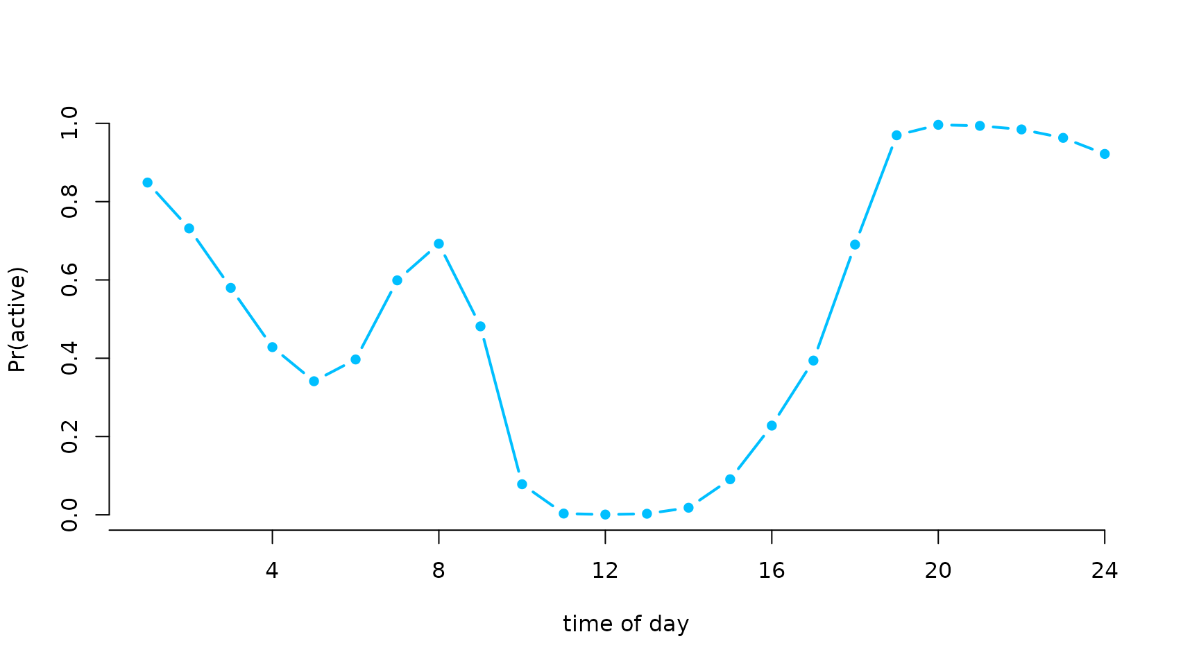
Smooth density estimation
To demonstrate nonparametric estimation of the state-dependent
densities, we will consider the nessi data set. It contains
acceleration data of the Loch Ness Monster, specifically the
overall dynamic body acceleration (ODBA). ODBA is
strictly positive with some very extreme values, making direct analysis
difficult. Hence, for our analysis we consider the logarithm of ODBA as
our observed process.
head(nessi)
#>         ODBA   logODBA state
#> 1 0.03775025 -3.276763     2
#> 2 0.05417830 -2.915475     2
#> 3 0.03625247 -3.317248     2
#> 4 0.01310802 -4.334531     1
#> 5 0.05402441 -2.918319     3
#> 6 0.06133794 -2.791357     3
hist(nessi$logODBA, prob = TRUE, breaks = 50, bor = "white",
     main = "", xlab = "log(ODBA)")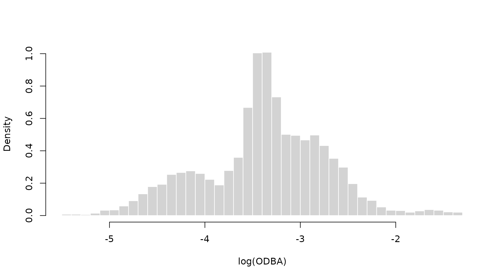
Clearly, there are at least three behavioural states in the data, and we start by fitting a simple 3-state Gaussian HMM with likelihood function:
nll = function(par){
    getAll(par, dat)
    sigma = exp(logsigma) # exp because strictly positive
    REPORT(mu); REPORT(sigma)
    Gamma = tpm(eta) # multinomial logit link
    delta = stationary(Gamma) # stationary dist of the homogeneous Markov chain
    allprobs = matrix(1, length(logODBA), N)
    ind = which(!is.na(logODBA))
    for(j in 1:N) allprobs[ind,j] = dnorm(logODBA[ind], mu[j], sigma[j])
    -forward(delta, Gamma, allprobs)
}
We then fit the model as explained in the vignette LaMa and RTMB.
# initial parameter list
par = list(mu = c(-4.5, -3.5, -2.5),
           logsigma = log(rep(0.5, 3)),
           eta = rep(-2, 6))

# data and hyperparameters
dat = list(logODBA = nessi$logODBA, N = 3)

# creating automatically differentiable objective function
obj = MakeADFun(nll, par, silent = TRUE)

# fitting the model
opt = nlminb(obj$par, obj$fn, obj$gr)

# reporting to get calculated quantities
mod = obj$report()

# visualising the results
color = c("orange", "deepskyblue", "seagreen3")
hist(nessi$logODBA, prob = TRUE, breaks = 50, bor = "white",
     main = "", xlab = "log(ODBA)")
for(j in 1:3) curve(mod$delta[j] * dnorm(x, mod$mu[j], mod$sigma[j]),
                    add = TRUE, col = color[j], lwd = 2, n = 500)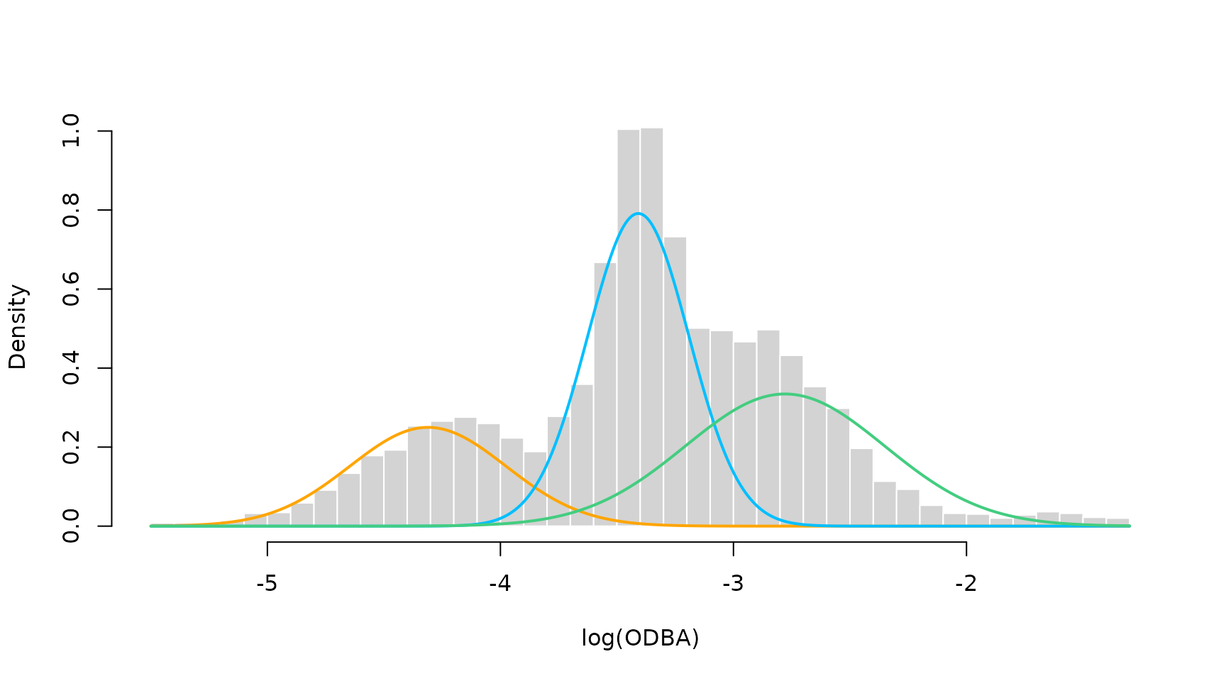
We see a clear lack-of-fit due to the inflexibility of the Gaussian state-dependent densities. Thus, we now fit a model with state-dependent densities based on P-Splines.
In a first step, this requires us to prepare the
design and penalty matrices needed
using smooth_dens_construct(). This function can take
multiple data streams and a set of initial parameters (specifying
initial means and standard deviations) for each data stream. It then
builds the P-Spline design and penalty matrices for
each data stream as well as a matrix of initial spline
coefficients based on the provided parameters. The basis
functions are standardised such that they integrate to one, which is
needed for density estimation.
# providing initial means and sds to initialise spline coefficients
par0 = list(logODBA = list(mean = c(-4, -3.3, -2.8), sd = c(0.3, 0.2, 0.5)))

# construct the smooth density objects
modmat = smooth_dens_construct(nessi["logODBA"], # only one data stream here
                               par = par0)
#> logODBA
#> Leaving out last column of the penalty matrix, fix the last spline coefficient at zero for identifiability!
#> Parameter matrix excludes the last column. Add a (fixed) zero column using 'cbind(coef, 0)' in your loss function!

# par is nested named list: top layer: each data stream
# for each data stream: initial means and standard deviations for each state

# objects for model fitting
Z = modmat$Z$logODBA # spline design matrix for logODBA
S = modmat$S$logODBA # penalty matrix for logODBA
beta = modmat$coef$logODBA # initial spline coefficients

# objects for prediction
Z_p = modmat$Z_predict$logODBA # prediction design matrix
xseq = modmat$xseq$logODBA # prediction sequence of logODBA values
Then, we can specify the penalised negative log-likelihood function.
The six lines in the middle are needed for P-Spline-based density
estimation. The coefficient matrix beta provided by
buildSmoothDens() has one column less than the number of
basis functions, which is also printed when calling
buildSmoothDens(). This is because the last column,
i.e. the last coefficient for each state, needs to be fixed to zero for
identifiability which we do by using
cbind(beta, 0). Then, we transform the unconstrained
parameter matrix to non-negative weights that sum to one (called
alpha) for each state using the inverse multinomial
logistic link (softmax). The columns of the allprobs matrix
are then computed as linear combinations of the columns of
Z and the weights alpha. Lastly, we penalise
the unconstrained coefficients beta (not the constrained
alpha’s) using the penalty() function.
pnll = function(par){
  getAll(par, dat)
  # regular stationary HMM stuff
  Gamma = tpm(eta)
  delta = stationary(Gamma)
  # smooth state-dependent densities
  alpha = exp(cbind(beta, 0))
  alpha = alpha / rowSums(alpha) # multinomial logit link
  REPORT(alpha)
  allprobs = matrix(1, nrow(Z), N)
  ind = which(!is.na(Z[,1])) # only for non-NA obs.
  allprobs[ind,] = Z[ind,] %*% t(alpha)
  # forward algorithm + penalty
  -forward(delta, Gamma, allprobs) +
    penalty(beta, S, lambda)
}
Now we specify the initial parameter and data list and fit the model.
In this case, we actually don’t need to add the observations to our
dat list anymore, as all the information is contained in
the design matrix Z.
par = list(beta = beta, # spline coefficients prepared by smooth_dens_construct()
           eta = rep(-2, 6)) # initial transition matrix on logit scale

dat = list(N = 3, # number of states
           Z = Z, # spline design matrix
           S = S, # spline penalty matrix
           lambda = rep(10, 3)) # initial penalty strength vector

# fitting the model using qREML
system.time(
  mod2 <- qreml(pnll, par, dat, random = "beta")
)
#> Creating AD function
#> Initialising with lambda: 10 10 10
#> outer 1 - lambda: 4.213 3.833 4.836
#> outer 2 - lambda: 2.309 1.937 3.045
#> outer 3 - lambda: 1.604 1.332 2.338
#> outer 4 - lambda: 1.305 1.127 2.028
#> outer 5 - lambda: 1.166 1.053 1.883
#> outer 6 - lambda: 1.099 1.026 1.812
#> outer 7 - lambda: 1.065 1.016 1.777
#> outer 8 - lambda: 1.048 1.012 1.76
#> outer 9 - lambda: 1.04 1.01 1.75
#> outer 10 - lambda: 1.035 1.01 1.747
#> outer 11 - lambda: 1.034 1.01 1.745
#> outer 12 - lambda: 1.033 1.01 1.745
#> outer 13 - lambda: 1.033 1.01 1.744
#> Converged
#> Final model fit with lambda: 1.033 1.01 1.744
#>    user  system elapsed
#>   8.617   3.461   7.965
After fitting the model, we can easily visualise the smooth densities
using the prepared prediction objects. We already have access to all
reported quantities because qreml() automatically runs the
reporting after model fitting.
sDens = Z_p %*% t(mod2$alpha) # all three state-dependent densities on a grid

hist(nessi$logODBA, prob = TRUE, breaks = 50, bor = "white", main = "", xlab = "log(ODBA)")
for(j in 1:3) lines(xseq, mod2$delta[j] * sDens[,j], col = color[j], lwd = 2)
lines(xseq, colSums(mod2$delta * t(sDens)), col = "black", lwd = 2, lty = 2)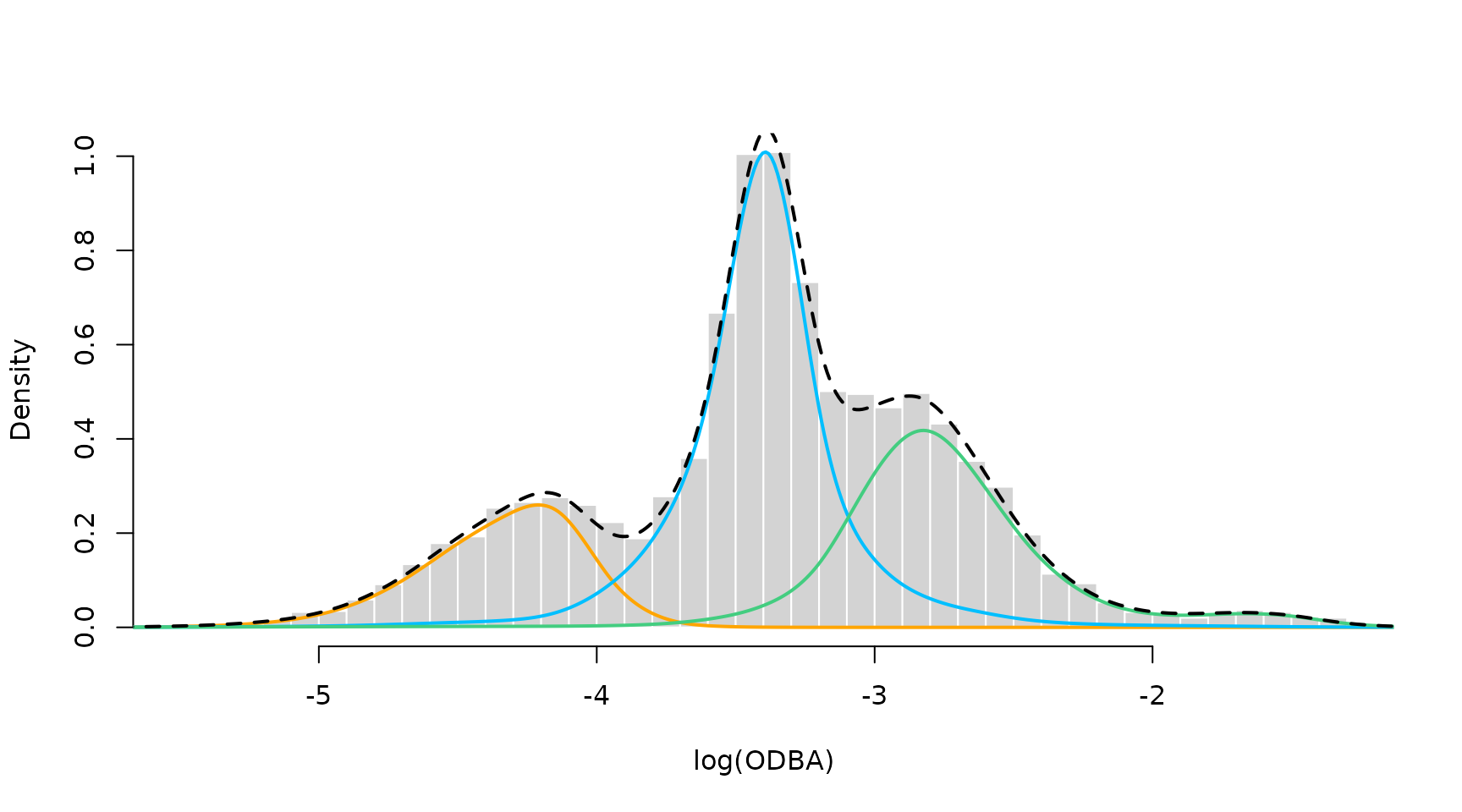
The P-Spline model results in a very good fit to the empirical distribution. This is because the first state has a skewed distribution, the second state has a high kurtosis and the third state has a funny right tail. The P-Spline model can capture all of these features where the parametric model failed to do so.
Markov-switching GAMLSS
Lastly, we want to demonstrate how one can easily fit
Markov-switching regression models where the state-dependent means and
potentially other parameters depend on covariates via smooth functions.
For this, we consider the energy data set contained in the
R package MSwM. It comprises 1784 daily observations of
energy prices (in Cents per kWh) in Spain which we want to explain using
the daily oil prices (in Euros per barrel) also provided in the data.
Specifically, we consider a 2-state MS-GAMLSS defined by
\text{price}_t \mid \{ S_t = i \} \sim N \bigl(\mu_t^{(i)},
(\sigma_t^{(i)})^2 \bigr),
\mu_t^{(i)} = \beta_{0,\mu}^{(i)} + s_{\mu}^{(i)}(\text{oil}_t), \quad
\text{log}(\sigma_t^{(i)}) = \beta_{0, \sigma}^{(i)} +
s_{\sigma}^{(i)}(\text{oil}_t), \quad i = 1,2,
not covering other potential explanatory covariates for the sake
of simplicity.
data(energy, package = "MSwM")
head(energy)
#>      Price      Oil      Gas     Coal   EurDol Ibex35   Demand
#> 1 3.188083 22.43277 14.40099 38.35157 1.134687 8.3976 477.3856
#> 2 4.953667 22.27263 19.02747 38.35157 1.106439 8.3771 609.1261
#> 3 4.730917 22.65383 18.48417 38.35157 1.106684 8.5547 650.3715
#> 4 4.531000 23.67657 18.30143 38.35157 1.116819 8.4631 647.0499
#> 5 5.141875 23.67209 14.55602 38.35157 1.122965 8.1773 627.9698
#> 6 6.322083 23.60534 15.22485 38.35157 1.122460 8.1866 693.2467
Similar to the first example, we can prepare the model matrices using
make_matrices():
modmat = make_matrices(~ s(Oil, k = 12, bs = "ps"), energy)
Z = modmat$Z # design matrix
S = modmat$S # penalty matrix (list)
Then, we specify the penalised negative log-likelihood function. It
differs from the first example as the state-dependent distributions, as
opposed to the state process parameters, depend on the covariate.
Additionally, we now have two completely separated spline-coefficient
matrices/ random effects called betaSpline and
alphaSpline for the state-dependent means and standard
deviations respectively. Thus, we need to pass them as a list to the
penalty() function.
We also pass the penalty matrix list S that is provided
by make_matrices(). This could potentially be a list of
length two if the two spline coefficient matrices were penalised
differently (e.g. by us using a different spline basis). In this case,
however, they are the same and we only pass the list of length one. It
does not matter to penalty() if we pass a list of length
one or just one matrix.
pnll = function(par) {
  getAll(par, dat)
  Gamma = tpm(eta) # computing the tpm
  delta = stationary(Gamma) # stationary distribution

  # regression parameters for mean and sd
  beta = cbind(beta0, betaSpline); REPORT(beta) # mean parameter matrix
  alpha = cbind(alpha0, alphaSpline); REPORT(alpha) # sd parameter matrix

  # calculating all covariate-dependent means and sds
  Mu = Z %*% t(beta) # mean
  Sigma = exp(Z %*% t(alpha)) # sd

  allprobs = cbind(dnorm(price, Mu[,1], Sigma[,1]),
                   dnorm(price, Mu[,2], Sigma[,2])) # state-dependent densities

  - forward(delta, Gamma, allprobs) +
    penalty(list(betaSpline, alphaSpline), S, lambda)
}
From this point on, the model fit is now basically identical to the
previous two examples. We specify initial parameters and include an
intial penalty strength parameter in the dat list.
# initial parameter list
par = list(eta = rep(-4, 2), # state process intercepts
           beta0 = c(2, 5), # state-dependent mean intercepts
           betaSpline = matrix(0, nrow = 2, ncol = 11), # mean spline coef
           alpha0 = c(0, 0), # state-dependent sd intercepts
           alphaSpline = matrix(0, nrow = 2, ncol = 11)) # sd spline coef

# data, model matrices and initial penalty strength
dat = list(price = energy$Price,
           Z = Z,
           S = S,
           lambda = rep(1e3, 4))

# model fit
system.time(
  mod3 <- qreml(pnll, par, dat, random = c("betaSpline", "alphaSpline"))
)
#> Creating AD function
#> Initialising with lambda: 1000 1000 1000 1000
#> outer 1 - lambda: 466.896 374.247 432.358 329.654
#> outer 2 - lambda: 250.283 143.698 200.372 113.051
#> outer 3 - lambda: 126.064 57.828 99.173 42.157
#> outer 4 - lambda: 72.846 26.191 56.901 18.27
#> outer 5 - lambda: 48.019 14.491 35.924 9.766
#> outer 6 - lambda: 35.991 10.081 24.159 6.518
#> outer 7 - lambda: 29.871 8.365 17.317 5.192
#> outer 8 - lambda: 26.631 7.684 13.359 4.626
#> outer 9 - lambda: 24.863 7.41 11.104 4.375
#> outer 10 - lambda: 23.88 7.297 9.836 4.263
#> outer 11 - lambda: 23.325 7.25 9.13 4.213
#> outer 12 - lambda: 23.007 7.23 8.74 4.189
#> outer 13 - lambda: 22.822 7.22 8.525 4.178
#> outer 14 - lambda: 22.719 7.216 8.406 4.173
#> outer 15 - lambda: 22.655 7.214 8.342 4.171
#> outer 16 - lambda: 22.618 7.213 8.305 4.17
#> outer 17 - lambda: 22.598 7.213 8.286 4.169
#> outer 18 - lambda: 22.589 7.212 8.279 4.169
#> outer 19 - lambda: 22.588 7.212 8.277 4.169
#> Converged
#> Final model fit with lambda: 22.588 7.212 8.277 4.169
#>    user  system elapsed
#>   8.283   4.691   7.321
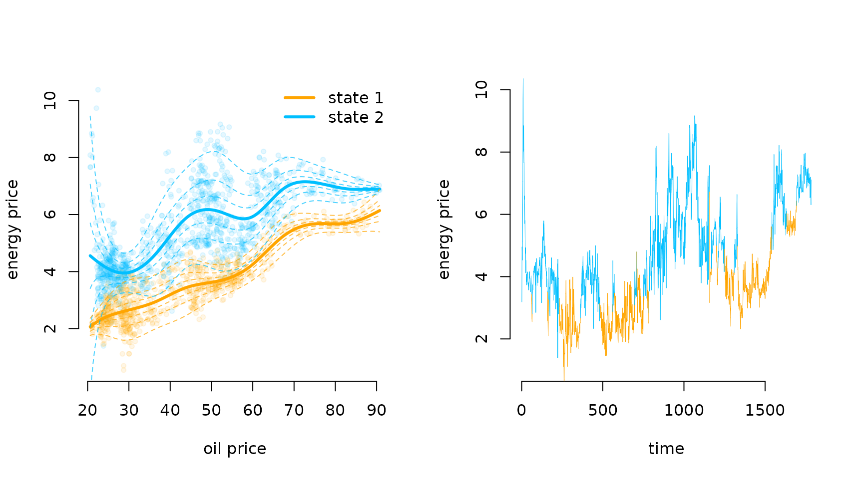
Having fitted the model, we can visualise the results. We first
decode the most probable state sequence and then plot the estimated
state-dependent densities as a function of the oil price, as well as the
decoded time series. For the former, we again create a fine grid of oil
price values and use predict() to build the associated
interpolating design matrix.
xseq = seq(min(energy$Oil), max(energy$Oil), length = 200) # sequence for prediction
Z_p = predict(modmat, newdata = data.frame(Oil = xseq)) # prediction design matrix

energy$states = viterbi(mod = mod3) # decoding most probable state sequence

Mu_plot = Z_p %*% t(mod3$beta)
Sigma_plot = exp(Z_p %*% t(mod3$alpha))

library(scales) # to make colors semi-transparent

par(mfrow = c(1,2))

# state-dependent distribution as a function of oil price
plot(energy$Oil, energy$Price, pch = 20, bty = "n", col = alpha(color[energy$states], 0.1),
     xlab = "oil price", ylab = "energy price")
for(j in 1:2) lines(xseq, Mu_plot[,j], col = color[j], lwd = 3) # means
qseq = qnorm(seq(0.5, 0.95, length = 4)) # sequence of quantiles
for(i in qseq){ for(j in 1:2){
  lines(xseq, Mu_plot[,j] + i * Sigma_plot[,j], col = alpha(color[j], 0.7), lty = 2)
  lines(xseq, Mu_plot[,j] - i * Sigma_plot[,j], col = alpha(color[j], 0.7), lty = 2)
}}
legend("topright", bty = "n", legend = paste("state", 1:2), col = color, lwd = 3)

# decoded time series
plot(NA, xlim = c(0, nrow(energy)), ylim = c(1,10), bty = "n",
     xlab = "time", ylab = "energy price")
segments(x0 = 1:(nrow(energy)-1), x1 = 2:nrow(energy),
         y0 = energy$Price[-nrow(energy)], y1 = energy$Price[-1],
         col = color[energy$states[-1]], lwd = 0.5)