Introduction to LaMa
Jan-Ole Koslik
Intro_to_LaMa.RmdThe R package LaMa provides convenient
functions for fitting a variety of latent Markov models
(Mews, Koslik, and
Langrock 2025), including hidden Markov
models (HMMs), hidden semi-Markov models
(HSMMs), state space models (SSMs) and
continuous-time variants via direct numerical
maximum likelihood estimation. The core idea is that the user
defines their own negative log-likelihood function for numerical
optimisation, but can rely on package functions for convenience and
speed.
The main families of functions are forward,
tpm and stationary and we showcase the
simplest versions in the following introductory example.
Introductory example: Homogeneous HMM
In this vignette, we start from the most simple HMM we can think of. Such a basic N-state HMM is a doubly stochastic process in discrete time. Observations are generated by one of N possible distributions f_j(x_t), j = 1, \dots N with an unobserved N-state Markov chain selecting which distribution is active at any given time point. Hence, HMMs can be interpreted as temporally dependent mixture models and are very popular across a wide range of disciplines like ecology, sports and finance where time-series data with underlying sequential dependencies are to be analysed. They statements above already hint at the two main assumptions in such a model, namely
- f(s_t \mid s_{t-1}, s_{t-2}, \dots, s_1) = f(s_t \mid s_{t-1}) (Markov assumption)
- f(x_t \mid x_1, \dots, x_{t-1}, x_{t-1}, x_T, s_1, \dots, s_T) = f(x_t \mid s_t) (conditional independence assumption).
The hidden state process is described by a Markov chain, as such a
stochastic process can easily be characterised by its initial
distribution \delta^{(1)} = (\Pr(S_1
= 1), \dots, \Pr(S_1 = N)) and the one-step transition
probabilities \gamma_{ij} = \Pr(S_t
= j \mid S_{t-1} = i), \quad i,j = 1, \dotsc, N which are
typically summarised in the so-called transition probability
matrix (t.p.m.) \Gamma =
(\gamma_{ij})_{i,j = 1, \dots, N} where row i is the conditional one-step ahead
distribution of the state process given that the current state is i. Such a matrix is most-conveniently
parameterised by an unconstrained parameter vector for the N (N-1) off-diagonal elements. Each row can
then be computed via the inverse multinomial logistic link (also known
as softmax). This can be done using the function tpm():
(Gamma = tpm(c(-2, -3))) # 2 states -> 2*(1-2) = 2 off-diagonal entries
#>           S1         S2
#> S1 0.9525741 0.04742587
#> S2 0.1192029 0.88079708
For HMMs with such homogeneous transition probabilities, we often
assume stationarity of the underlying Markov chain, as
well-behaved Markov chains converge to a unique stationary distribution.
When we e.g. observe an animal and model its behavioral states by a
Markov chain, it is reasonable to assume that the chain has been running
for a long time prior to our observation and thus already converged to
its stationary distribution. This distribution (which we call \delta) can be computed by solving the system
of equations
\delta \Gamma = \delta, \quad \text{s.t.} \; \sum_{j=1}^N \delta_j = 1,
which is implemented in the function stationary().
For stationary HMMs, we then replace the initial distribution \delta^{(1)} by this stationary distribution.
We can easily compute the stationary distribution associated with the
above t.p.m. using
(delta = stationary(Gamma))
#>        S1        S2
#> 0.7153801 0.2846199
This stationary distribution can be interpreted as the log-run-time proportion of time spent in each state.
For the conditional distributions of the observations f_j(x_t), a typical choice would be some kind of parametric family like normal or gamma distributions with state-specific means and standard deviations. For a more exhaustive description of such models see Zucchini, MacDonald, and Langrock (2016).
Generating data from a 2-state HMM
We start by simulating some data from a simple 2-state HMM with
Gaussian state-dependent distributions, to get some intuition. Here we
can again use stationary() to compute the stationary
distribution.
# parameters
mu = c(0, 6)    # state-dependent means
sigma = c(2, 4) # state-dependent standard deviations
Gamma = matrix(c(0.95, 0.05, 0.15, 0.85), # transition probability matrix
               nrow = 2, byrow = TRUE)
delta = stationary(Gamma) # stationary distribution

# simulation
n = 1000
set.seed(123)
s = rep(NA, n)
s[1] = sample(1:2, 1, prob = delta) # sampling first state from delta
for(t in 2:n){
  # drawing the next state conditional on the last one
  s[t] = sample(1:2, 1, prob = Gamma[s[t-1],])
}
# drawing the observation conditional on the states
x = rnorm(n, mu[s], sigma[s])

color = c("orange", "deepskyblue")
plot(x[1:200], bty = "n", pch = 20, ylab = "x",
     col = color[s[1:200]])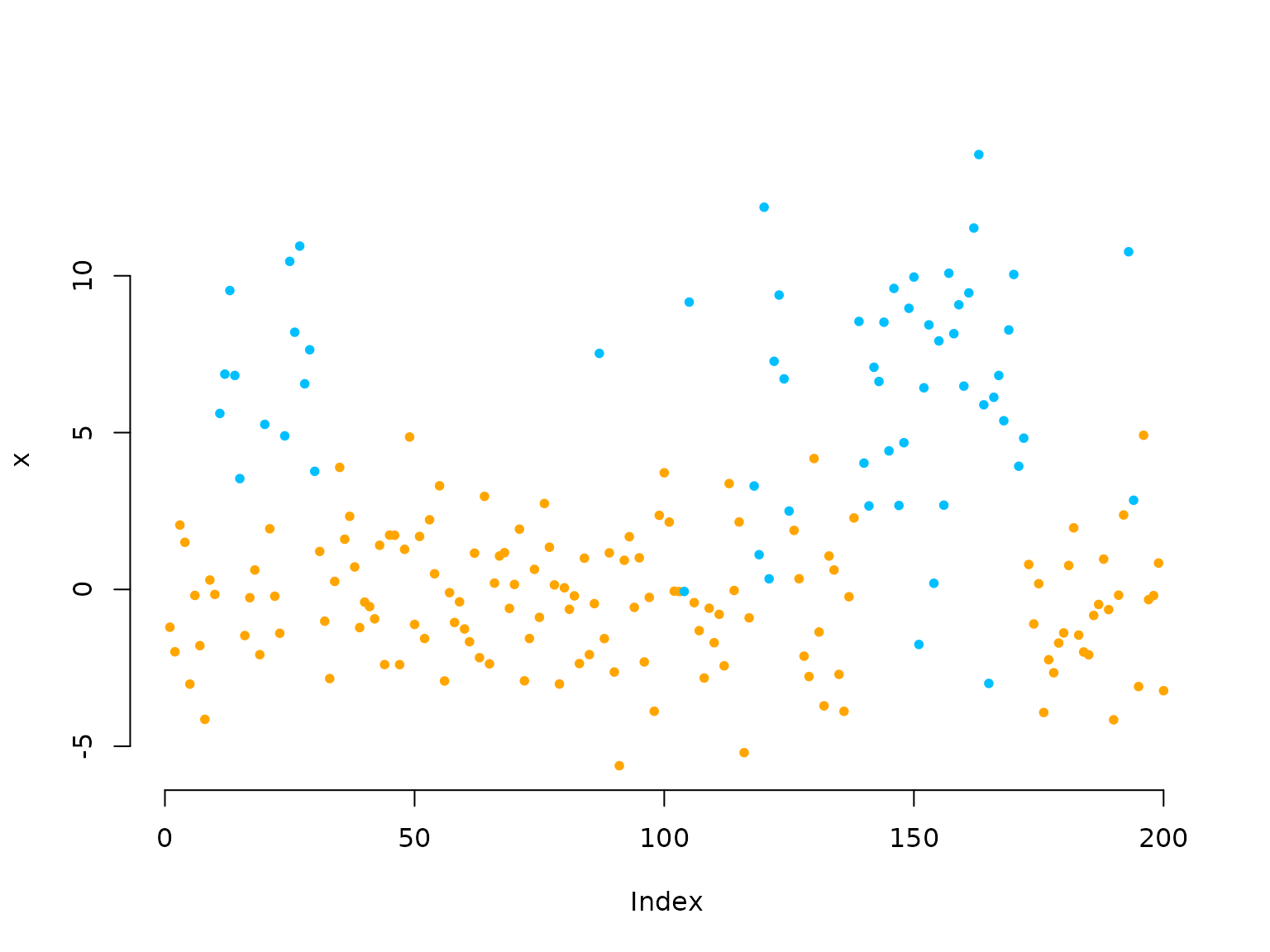
Inference by direct numerical maximum likelihood estimation
Inference for HMMs is more difficult compared to e.g. regression modelling as the observations are not independent. We want to estimate model parameters via maximum likelihood estimation, due to the nice properties possessed by the maximum likelihood estimator. However, computing the HMM likelihood for observed data points x_1, \dots, x_T is a non-trivial task as we do not observe the underlying states. We thus need to sum out all possible state sequences which would be infeasible for general state processes. We can, however, exploit the Markov property and thus calculate the likelihood recursively as a matrix product using the so-called forward algorithm. In closed form, the HMM likelihood then becomes
L(\theta) = \delta^{(1)} P(x_1) \Gamma P(x_2) \Gamma \dots \Gamma P(x_T)
1^t,
where \delta^{(1)} and \Gamma are as defined above, P(x_t) is a diagonal matrix with
state-dependent densities or probability mass functions f_j(x_t) = f(x_t \mid S_t = j) on its
diagonal and 1 is a row vector of ones
with length N. All model parameters are
here summarised in the vector \theta.
Being able to evaluate the likelihood function, it can be numerically
maximised by popular optimisers like nlm() or
optim().
The algorithm explained above suffers from numerical underflow and
for T only moderately large the
likelihood is rounded to zero. Thus, one can use a scaling strategy,
detailed by Zucchini, MacDonald, and Langrock (2016), to avoid this and calculate the
log-likelihood recursively. This version of the forward algorithm is
implemented in LaMa and written in C++.
Additionally, for HMMs we often need to constrain the domains of
several of the model parameters in \theta (i.e. positive standard deviations or
a transition probability matrix with elements between 0 and 1 and rows
that sum to one). One could now resort to constrained numerical
optimisation but in practice the better option is to maximise the
likelihood w.r.t. a transformed version (to the real number line) of the
model parameters by using suitable invertible and differentiable link
functions (denoted by par in the code). For example we use
the log-link for parameters that need to be strictly positive and the
multinomial logistic link for the transition probability matrix. While
the former can easily be coded by hand, the latter is implemented in the
functions of the tpm family for convenience and
computational speed.
For efficiency, it is also advisable to evaluate the state-dependent
densities (or probability mass functions) vectorised outside the
recursive forward algorithm. This results in a matrix containing the
state-dependent likelihoods for each data point (rows), conditional on
each state (columns), which, throughout the package, we call the
allprobs matrix.
In this example, within the negative log-likelihood function we build
the homogeneous transition probability matrix using the
tpm() function and compute the stationary distribution of
the Markov chain using stationary(). We then build the
allprobs matrix and calculate the log-likelihood using
forward() in the last line. It is returned negative such
that the function can be numerically minimised by
e.g. nlm().
nll = function(par, x){
  # parameter transformations for unconstrained optimisation
  Gamma = tpm(par[1:2]) # multinomial logistic link
  delta = stationary(Gamma) # stationary initial distribution
  mu = par[3:4] # no transformation needed
  sigma = exp(par[5:6]) # strictly positive
  # calculating all state-dependent probabilities outside the forward algorithm
  allprobs = matrix(1, length(x), 2)
  for(j in 1:2) allprobs[,j] = dnorm(x, mu[j], sigma[j])
  # return negative for minimisation
  -forward(delta, Gamma, allprobs)
}
Fitting an HMM to the data
par = c(logitGamma = qlogis(c(0.05, 0.05)),
        mu = c(1,4),
        logsigma = c(log(1),log(3)))
# initial transformed parameters: not chosen too well
system.time(
  mod <- nlm(nll, par, x = x)
)
#>    user  system elapsed
#>   0.125   0.010   0.134
We see that implementation of the forward algorithm in C++ leads to really fast estimation speeds.
Visualising results
After model estimation, we need to retransform the unconstrained parameters according to the code inside the likelihood:
# transform parameters to working
Gamma = tpm(mod$estimate[1:2])
delta = stationary(Gamma) # stationary HMM
mu = mod$estimate[3:4]
sigma = exp(mod$estimate[5:6])

hist(x, prob = TRUE, bor = "white", breaks = 40, main = "")
curve(delta[1]*dnorm(x, mu[1], sigma[1]), add = TRUE, lwd = 2, col = "orange", n=500)
curve(delta[2]*dnorm(x, mu[2], sigma[2]), add = TRUE, lwd = 2, col = "deepskyblue", n=500)
curve(delta[1]*dnorm(x, mu[1], sigma[1])+delta[2]*dnorm(x, mu[2], sigma[2]),
      add = TRUE, lwd = 2, lty = "dashed", n=500)
legend("topright", col = c(color, "black"), lwd = 2, bty = "n",
       lty = c(1,1,2), legend = c("state 1", "state 2", "marginal"))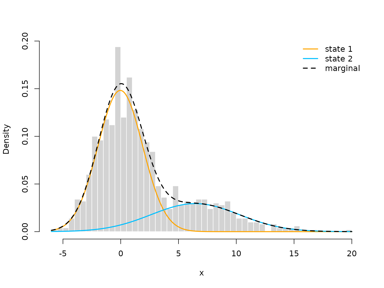
We can also decode the most probable state sequence with the
viterbi() function, when first computing the
allprobs matrix:
allprobs = matrix(1, length(x), 2)
for(j in 1:2) allprobs[,j] = dnorm(x, mu[j], sigma[j])

states = viterbi(delta, Gamma, allprobs)

plot(x, pch = 20, bty = "n", col = color[states])
legend("topright", pch = 20, legend = c("state 1", "state 2"),
       col = color, box.lwd = 0)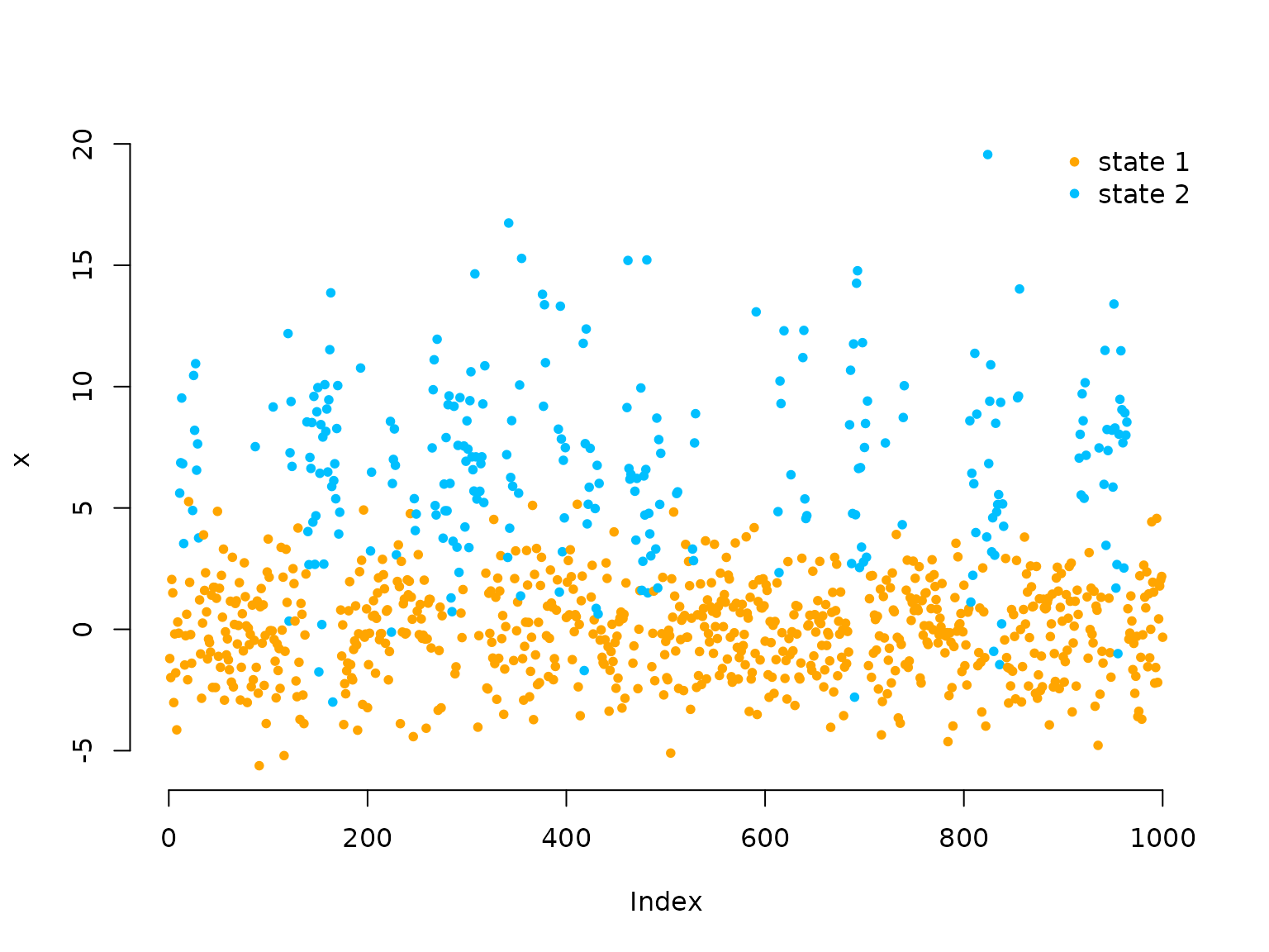
Lastly, we can do some model checking using pseudo-residuals. First, we need to compute the local state probabilities of our observations:
probs = stateprobs(delta, Gamma, allprobs)Then, we can pass the observations, the state probabilities, the
parametric family and the estimated parameters to the
pseudo_res() function to get pseudo-residuals for model
validation. These should be standard normally distributed if the model
is correct.
pres = pseudo_res(x, # observations
                  "norm", # parametric distribution to use
                  list(mean = mu, sd = sigma), # parameters for that distribution
                  probs) # local state probabilities

# use the plotting method for LaMaResiduals
plot(pres, hist = TRUE)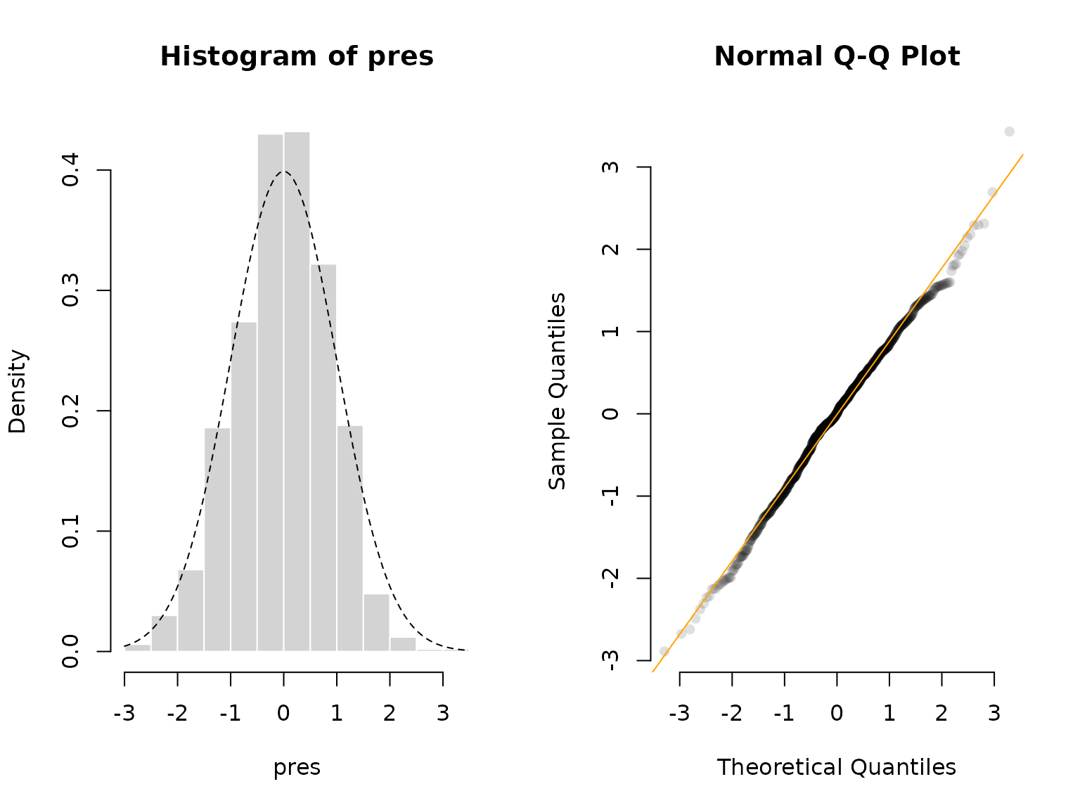
In this case, our model looks really good – as it should because we simulated from the exact same model.
Continue reading with LaMa and RTMB, Inhomogeneous HMMs, Periodic HMMs, Longitudinal data, State-space models, Hidden semi-Markov models, or Continuous-time HMMs.