Periodic HMMs

Before diving into this vignette, we recommend reading the vignettes Introduction to LaMa and Inhomogeneous HMMs.

This vignette shows how to fit HMMs where the state process is a periodically inhomogeneous Markov chain. Formally, this means that for all $t$

$\Gamma^{(t+L)} = \Gamma^{(t)},$ where $\Gamma^{(t)}$ is the transition probability matrix at time $t$ and $L$ is the cycle length. Such a setting can conveniently modelled by letting the off-diagonal elements be trigonometric functions of a cyclic variable such as time of day. While this model is a special case of the general, inhomogeneous HMM, it is often more interpretable and very important in statistical ecology, hence we discuss it separately.

# loading the package
library(LaMa)
#> Loading required package: RTMB

Setting parameters for simulation

We simulate a 2-state HMM with Gaussian state-dependent distributions. For the periodic inhomogeneity, we choose a bimodal activity pattern. All $L$ transition probability matrices can conveniently be calculated using tpm_p(). Under the hood, this performs a basis expansion using trigBasisExp() into sine and cosine terms and uses linear predictos of the form $\eta^{(t)}_{ij} = \beta_0^{(ij)} + \sum_{k=1}^K \bigl( \beta_{1k}^{(ij)} \sin(\frac{2 \pi k t}{L}) + \beta_{2k}^{(ij)} \cos(\frac{2 \pi k t}{L}) \bigr)$ for the off-diagonal entries of the transition probability matrix. The special case of periodically inhomogeneous Markov chains also allows the derivation of a so-called periodically stationary distribution (Koslik et al. 2023) which we can compute this distribution using stationary_p().

# parameters
mu = c(4, 14)   # state-dependent means
sigma = c(3, 5) # state-dependent standard deviations

L = 48 # half-hourly data: 48 observations per day
beta = matrix(c(-1, 1, -1, -1, 1,
                -2, -1, 2, 2, -2), nrow = 2, byrow = TRUE)
Gamma = tpm_p(seq(1, 48, by = 1), L, beta, degree = 2)
Delta = stationary_p(Gamma)

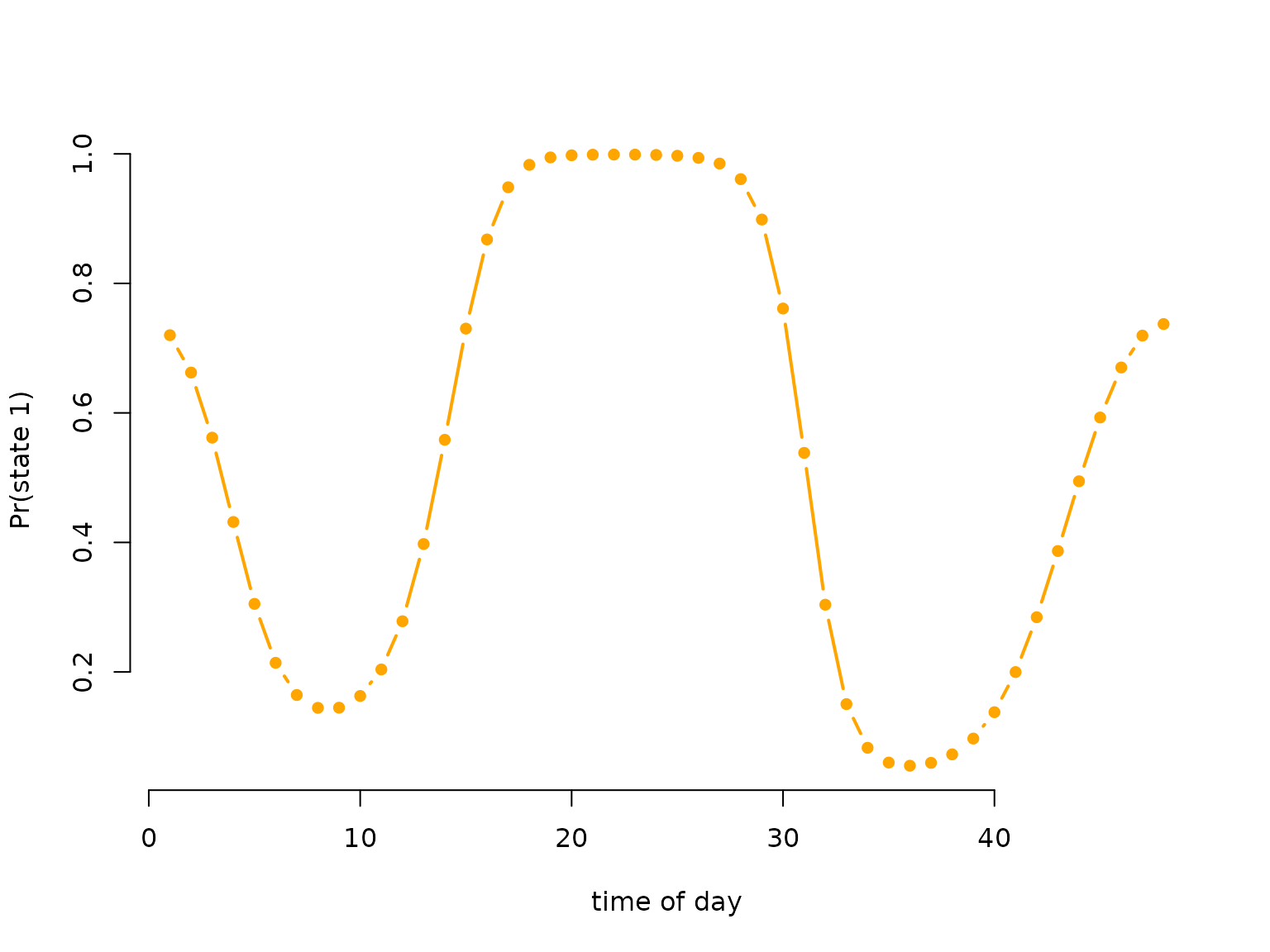
# having a look at the periodically stationary distribution
color = c("orange", "deepskyblue")
plot(Delta[,1], type = "b", lwd = 2, pch = 16, col = color[1], bty = "n", 
     xlab = "time of day", ylab = "Pr(state 1)")

# only plotting one state, as the other probability is just 1-delta

Simulating data

# simulation
tod = rep(1:48, 50) # time of day variable, 50 days
n = length(tod)
set.seed(123)
s = rep(NA, n)
s[1] = sample(1:2, 1, prob = Delta[tod[1],]) # initial state from stationary dist
for(t in 2:n){
  # sampling next state conditional on previous one and the periodic t.p.m.
  s[t] = sample(1:2, 1, prob = Gamma[s[t-1],,tod[t]])
}
# sampling observations conditional on the states
x = rnorm(n, mu[s], sigma[s])

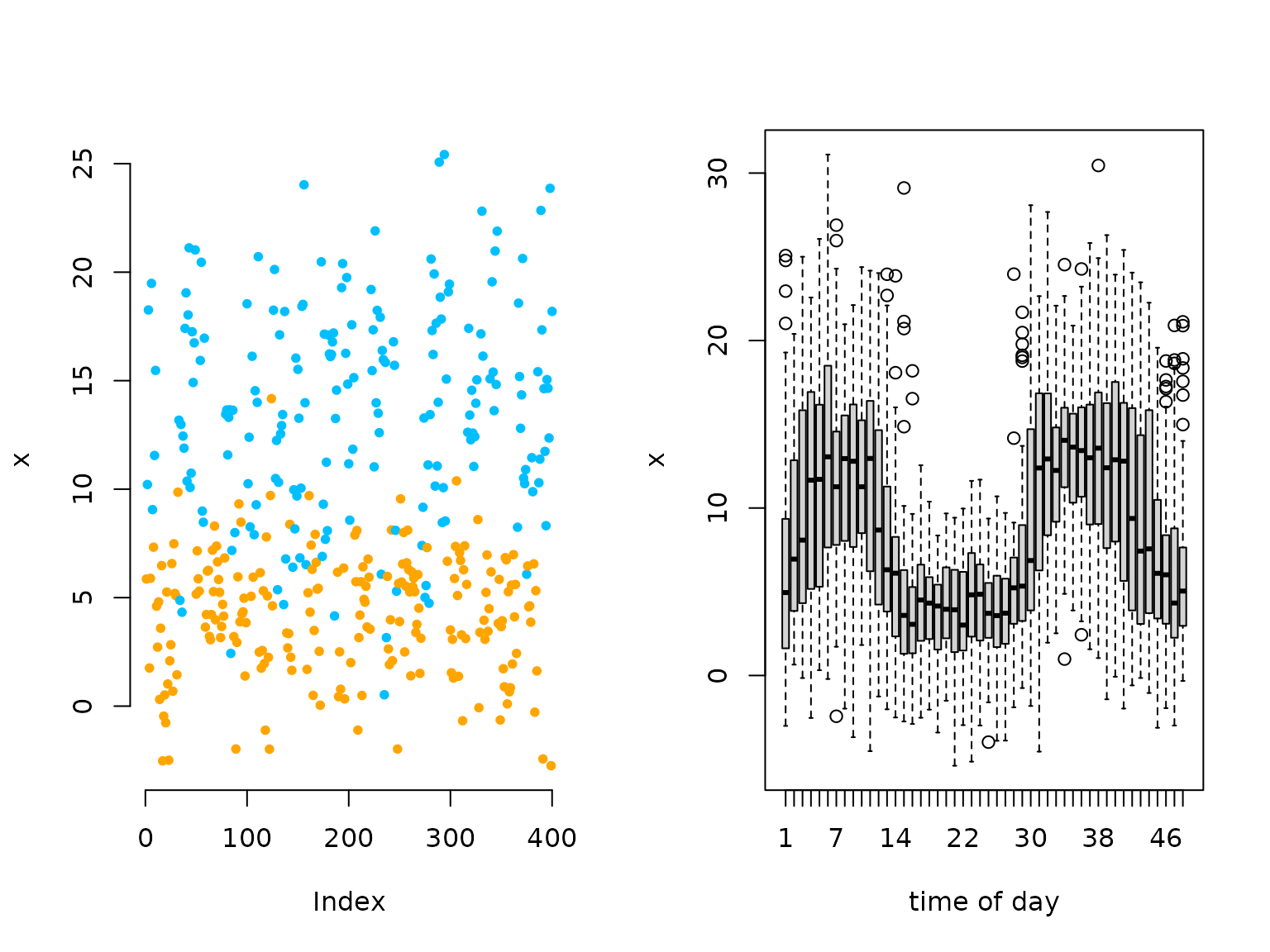
oldpar = par(mfrow = c(1,2))
plot(x[1:400], bty = "n", pch = 20, ylab = "x", 
     col = color[s[1:400]])
boxplot(x ~ tod, xlab = "time of day")

# we see a periodic pattern in the data
par(oldpar)

Trigonometric modeling of the transition probalities

Writing the negative log-likelihood function

We specify the likelihood function and pretend we know the degree of the trigonometric link which, in practice, is never the case. Again we use tpm_p() and we compute the periodically stationary start by using stationary_p() with the additional argument that specifies which time point to compute.

nll = function(par, x, tod){
  beta = matrix(par[1:10], nrow = 2) # matrix of coefficients
  Gamma = tpm_p(tod = 1:48, L = 48, beta = beta, degree = 2) # calculating all L tpms
  delta = stationary_p(Gamma, t = tod[1]) # periodically stationary start
  mu = par[11:12]
  sigma = exp(par[13:14])
  # calculate all state-dependent probabilities
  allprobs = matrix(1, length(x), 2)
  for(j in 1:2) allprobs[,j] = dnorm(x, mu[j], sigma[j])
  # return negative for minimization
  -forward_p(delta, Gamma, allprobs, tod)
}

Fitting an HMM to the data

par = c(beta = c(-1,-2, rep(0, 8)), # starting values state process
        mu = c(4, 14), # initial state-dependent means
        logsigma = c(log(3),log(5))) # initial state-dependent sds
system.time(
  mod <- nlm(nll, par, x = x, tod = tod)
)
#>    user  system elapsed 
#>   0.769   0.007   0.776

Visualising results

Again, we use tpm_p() and stationary_p() to tranform the parameters.

# transform parameters to working
beta_hat = matrix(mod$estimate[1:10], nrow = 2)
Gamma_hat = tpm_p(tod = 1:48, L = 48, beta = beta_hat, degree = 2)
Delta_hat = stationary_p(Gamma_hat)
mu_hat = mod$estimate[11:12]
sigma_hat = exp(mod$estimate[13:14])

delta_hat = apply(Delta_hat, 2, mean)

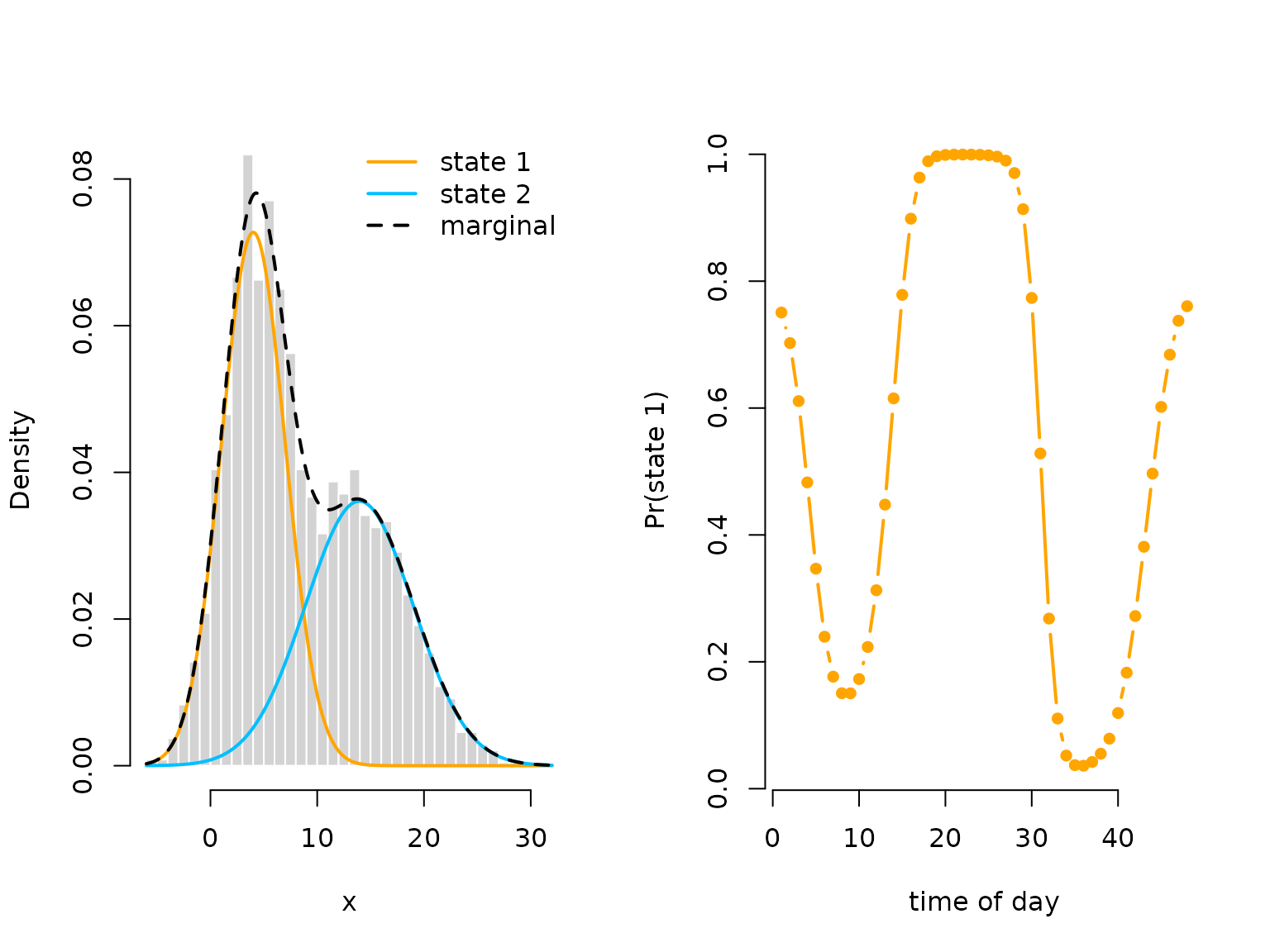
oldpar = par(mfrow = c(1,2))
hist(x, prob = TRUE, bor = "white", breaks = 40, main = "")
curve(delta_hat[1]*dnorm(x, mu_hat[1], sigma_hat[1]), add = TRUE, lwd = 2, 
      col = color[1], n=500)
curve(delta_hat[2]*dnorm(x, mu_hat[2], sigma_hat[2]), add = TRUE, lwd = 2, 
      col = color[2], n=500)
curve(delta_hat[1]*dnorm(x, mu_hat[1], sigma_hat[1])+
        delta_hat[2]*dnorm(x, mu[2], sigma_hat[2]),
      add = TRUE, lwd = 2, lty = "dashed", n = 500)
legend("topright", col = c(color[1], color[2], "black"), lwd = 2, bty = "n",
       lty = c(1,1,2), legend = c("state 1", "state 2", "marginal"))

plot(Delta_hat[,1], type = "b", lwd = 2, pch = 16, col = color[1], bty = "n", 
     xlab = "time of day", ylab = "Pr(state 1)")

par(oldpar)

References

Koslik, Jan-Ole, Carlina C Feldmann, Sina Mews, Rouven Michels, and Roland Langrock. 2023. “Inference on the State Process of Periodically Inhomogeneous Hidden Markov Models for Animal Behavior.” arXiv Preprint arXiv:2312.14583.