State-space models

Jan-Ole Koslik

Before diving into this vignette, we recommend reading the vignette Introduction to LaMa.

This vignette shows how to fit state-space models which can be interpreted as generalisation of HMMs to continuous state spaces. Several approaches exist to fitting such models, but Langrock (2011) showed that very general state-space models can be fitted via approximate maximum likelihood estimation, when the continous state space is finely discretised. This is equivalent to numerical integration over the state process using midpoint quadrature.

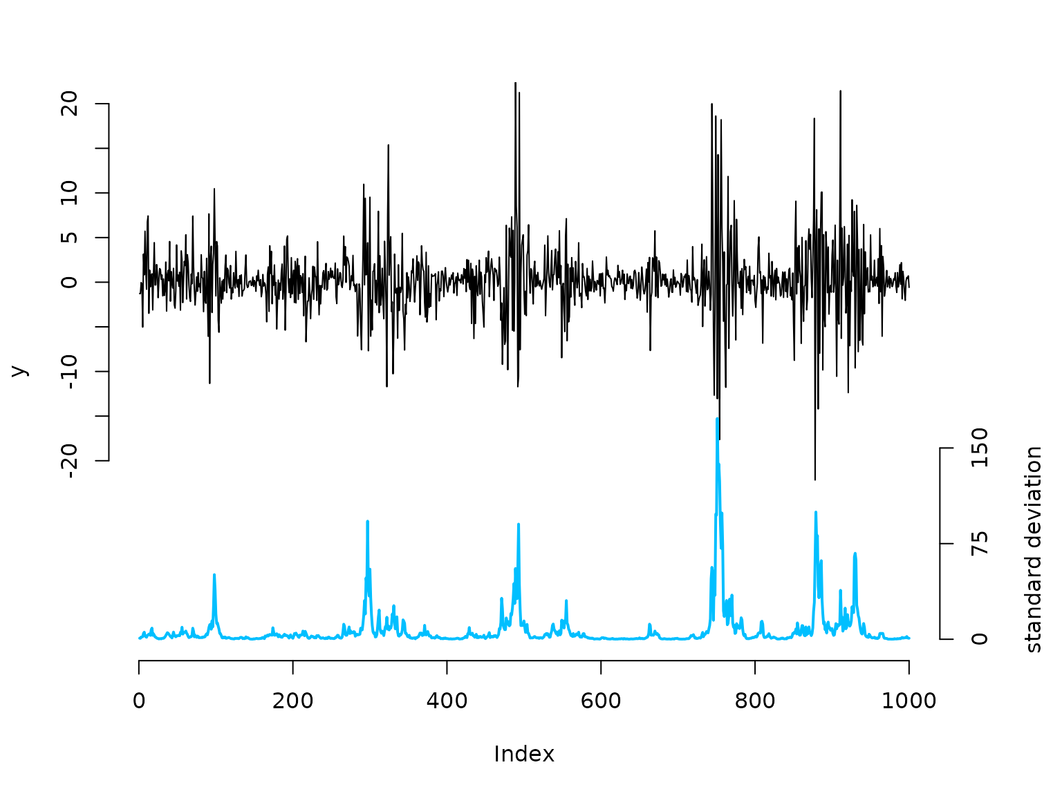
Here, we will showcase this approach for a basic stochastic volatily model which, while being very simple, captures most of the stylised facts of financial time series. In this model the unobserved marked volatility is described by an AR(1) process:

$$g_t = \phi g_{t-1} + \sigma \eta_t, \qquad \eta_t \sim N(0,1),$$ with autoregression parameter $\phi < 1$ and dispersion parameter $\sigma$. Share returns $y_t$ can then be modelled as $$y_t = \beta \epsilon_t \exp(g_t / 2),$$ where $\epsilon_t \sim N(0,1)$ and $\beta > 0$ is the baseline standard deviation of the returns (when $g_t$ is in equilibrium), which implies $$y_t \mid g_t \sim N(0, (\beta e^{g_t / 2})^2).$$

Simulating data from the stochastic volatility model

We start by simulating data from the above specified model:

# loading the package
library(LaMa)
#> Loading required package: RTMB

beta = 2 # baseline standard deviation
phi = 0.95 # AR parameter of the log-volatility process
sigma = 0.5 # variability of the log-volatility process

n = 1000
set.seed(123)
g = rep(NA, n)
g[1] = rnorm(1, 0, sigma / sqrt(1-phi^2)) # stationary distribution of AR(1) process
for(t in 2:n){
  # sampling next state based on previous state and AR(1) equation
  g[t] = rnorm(1, phi*g[t-1], sigma)
}
# sampling zero-mean observations with standard deviation given by latent process
y = rnorm(n, 0, beta * exp(g/2)) 

# share returns
oldpar = par(mar = c(5,4,3,4.5)+0.1)
plot(y, type = "l", bty = "n", ylim = c(-40,20), yaxt = "n")
# true underlying standard deviation
lines(beta*exp(g)/7 - 40, col = "deepskyblue", lwd = 2)
axis(side=2, at = seq(-20,20,by=5), labels = seq(-20,20,by=5))
axis(side=4, at = seq(0,150,by=75)/7-40, labels = seq(0,150,by=75))
mtext("standard deviation", side=4, line=3, at = -30)

par(oldpar)

Writing the negative log-likelihood function

To calculate the likelihood, we need to integrate over the state space. We approximate this high-dimensional integral using a midpoint quadrature which ultimately results in a fine discretisation of the continuous state space into the intervals b with width h and midpoints bstar (Langrock 2011). Thus, the likelihood below corresponds to a basic HMM likelihood with a large number of states.

nll = function(par, y, bm, m){
  phi = plogis(par[1])
  sigma = exp(par[2])
  beta = exp(par[3])
  b = seq(-bm, bm, length = m+1) # intervals for midpoint quadrature
  h = b[2] - b[1] # interval width
  bstar = (b[-1] + b[-(m+1)]) / 2 # interval midpoints
  # approximating t.p.m. resulting from midpoint quadrature
  Gamma = sapply(bstar, dnorm, mean = phi * bstar, sd = sigma) * h
  delta = h * dnorm(bstar, 0, sigma / sqrt(1-phi^2)) # stationary distribution
  # approximating state-dependent density based on midpoints
  allprobs = t(sapply(y, dnorm, mean = 0, sd = beta * exp(bstar/2)))
  # forward algorithm
  -forward(delta, Gamma, allprobs)
}

Fitting an SSM to the data

par = c(qlogis(0.95), log(0.3), log(1))
bm = 5 # relevant range of underlying volatility (-5,5)
m = 100 # number of approximating states

system.time(
  mod <- nlm(nll, par, y = y, bm = bm, m = m)
)
#>    user  system elapsed 
#>   1.503   2.299   0.977

Results

## parameter estimates
(phi = plogis(mod$estimate[1]))
#> [1] 0.9516567
(sigma = exp(mod$estimate[2]))
#> [1] 0.4436876
(beta = exp(mod$estimate[3]))
#> [1] 2.184006

## decoding states
b = seq(-bm, bm, length = m+1) # intervals for midpoint quadrature
h = b[2]-b[1] # interval width
bstar = (b[-1] + b[-(m+1)])/2 # interval midpoints
Gamma = sapply(bstar, dnorm, mean = phi*bstar, sd = sigma) * h
delta = h * dnorm(bstar, 0, sigma/sqrt(1-phi^2)) # stationary distribution
# approximating state-dependent density based on midpoints
allprobs = t(sapply(y, dnorm, mean = 0, sd = beta * exp(bstar/2)))

# actual decoding
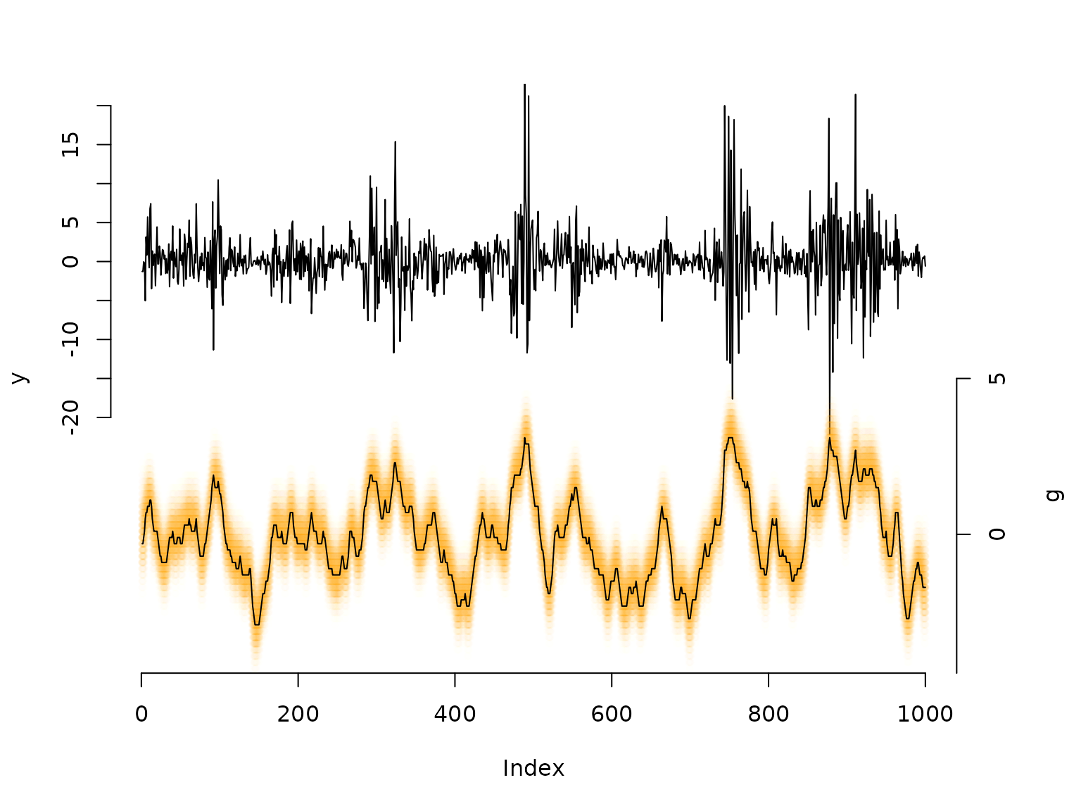
probs = stateprobs(delta, Gamma, allprobs) # local/ soft decoding
states = viterbi(delta, Gamma, allprobs) # global/ hard decoding

oldpar = par(mar = c(5,4,3,4.5)+0.1)
plot(y, type = "l", bty = "n", ylim = c(-50,20), yaxt = "n")
# when there are so many states it is not too sensable to only plot the most probable state,
# as its probability might still be very small. Generally, we are approximating continuous 
# distributions, thus it makes sense to plot the entire conditional distribution.
maxprobs = apply(probs, 1, max)
for(t in 1:nrow(probs)){
  colend = round((probs[t,]/(maxprobs[t]*5))*100)
  colend[which(colend<10)] = paste0("0", colend[which(colend<10)])
  points(rep(t, m), bstar*4-35, col = paste0("#FFA200",colend), pch = 20)
}
# we can add the viterbi decoded volatility levels as a "mean"
lines(bstar[states]*4-35)

axis(side=2, at = seq(-20,20,by=5), labels = seq(-20,20,by=5))
axis(side=4, at = seq(-5,5, by = 5)*4-35, labels = seq(-5,5, by = 5))
mtext("g", side=4, line=3, at = -30)

par(oldpar)

References

Langrock, Roland. 2011. “On Some Special-Purpose Hidden Markov Models.” PhD thesis, University of Göttingen.