Inhomogeneous HMMs
Jan-Ole Koslik
Inhomogeneous_HMMs.RmdBefore diving into this vignette, we recommend reading the vignette Introduction to LaMa.
This vignette explains how to fit inhomogeneous HMMs, i.e. models
that depend on external covariates with LaMa. Such
inhomogeneity in HMMs can result from covariates affecting the
transition probabilities of the underlying Markov chain, or covariates
affecting the state-dependent distributions, which would then be called
Markov-switching regression. We will begin with effects in the state
process
Covariate effects in the state process
If covariates affect the transition probabilities, this implies that
we model the transition probability matrix as a function of said
covariates. Let z_t be a vector of
covariates of length p+1 for t = 1, \dots, T, where the first entry is
always equal to 1 to include an
intercept. Moreover, let \beta_{ij} be
a vector of regression parameters, also of length p+1 for each off-diagonal element (i \neq j) of the transition probability
matrix. First, consider linear predictors
\eta_{ij}^{(t)} = \beta_{ij}^{'} z_t,
for t = 1, \dots, T. As the
transition probabilities need to be in lie in the interval (0,1) and each row of the transition matrix
needs to sum to one, we obtain the transition probabilities via the
inverse multinomial logistic link as
\gamma_{ij}^{(t)} = \Pr(S_t = j \mid S_{t-1} = i) =
\frac{\exp(\eta_{ij}^{(t)})}{\sum_{k=1}^N \exp(\eta_{ik}^{(t)})},
where \eta_{ii} is set to zero
for i = 1, \dots, N for identifiability
and N is the number of hidden states.
The function tpm_g() conducts this calculation for all
elements of the t.p.m. and all time points efficiently in C++.
At this point we want to point out that the definition of the
transition probabilities is not necessarily unique. Indeed for data
points at times 1, \dots, T we only
need T-1 transition probability
matrices. The definition above means that the transition probability
between t-1 and t depends on the covariate values at time
point t, but we could also have defined
\gamma_{ij}^{(t)} = \Pr(S_{t+1} = j \mid S_t = i).
We want to point out that these two specifications are
not equivalent. For HMMs there is no established
convention, so this choice needs to be made by users and can be
important when the exact timing of the covariate effect is relevant. In
LaMa this comes down to either passing the design matrix
excluding its first or last row to tpm_g(), where we use
the first option in this vignette. If you forget to exclude the first or
the last row of the design matrix when calculating all transition
matrices, and pass an array of dimension c(N,N,T) to
forward_g() for likelihood evaluation, the function will
revert to the first option by just ignoring the first slice of the
array.
Simulation example
We begin by simulating data from the above specified model, assuming
2 states and Gaussian state-dependent distributions. The covariate
effects for the state process are fully specified by a parameter matrix
beta of dimension c(N*(N-1), p+1). By default
the function tpm_g() will fill the off-diagonal elements of
each transition matrix by column, which can be changed by setting
byrow = TRUE. The latter is useful, as popular HMM packages
like moveHMM or momentuHMM return the
parameter matrix such that the t.p.m. needs to be filled by row.
# parameters
mu = c(5, 20)   # state-dependent means
sigma = c(4, 5) # state-dependent standard deviations

# state process regression parameters
beta = matrix(c(-2, -2,       # intercepts
                -1, 0.5,      # linear effects
                0.25, -0.25), # quadratic effects
              nrow = 2)

n = 1000 # number of observations
set.seed(123)
z = rnorm(n) # in practice there will be n covariate values.
# However, we only have n-1 transitions, therefore we only need n-1 values:
Z = cbind(z, z^2) # quadratic effect of z
Gamma = tpm_g(Z = Z[-1,], beta) # of dimension c(2, 2, n-1)
delta = c(0.5, 0.5) # non-stationary initial distribution

color = c("orange", "deepskyblue")

oldpar = par(mfrow = c(1,2))
zseq = seq(-2,2,by = 0.01)
Gamma_seq = tpm_g(Z = cbind(zseq, zseq^2), beta)
plot(zseq, Gamma_seq[1,2,], type = "l", lwd = 3, bty = "n", ylim = c(0,1),
     xlab = "z", ylab = "gamma_12", col = color[1])
plot(zseq, Gamma_seq[2,1,], type = "l", lwd = 3, bty = "n", ylim = c(0,1),
     xlab = "z", ylab = "gamma_21", col = color[2])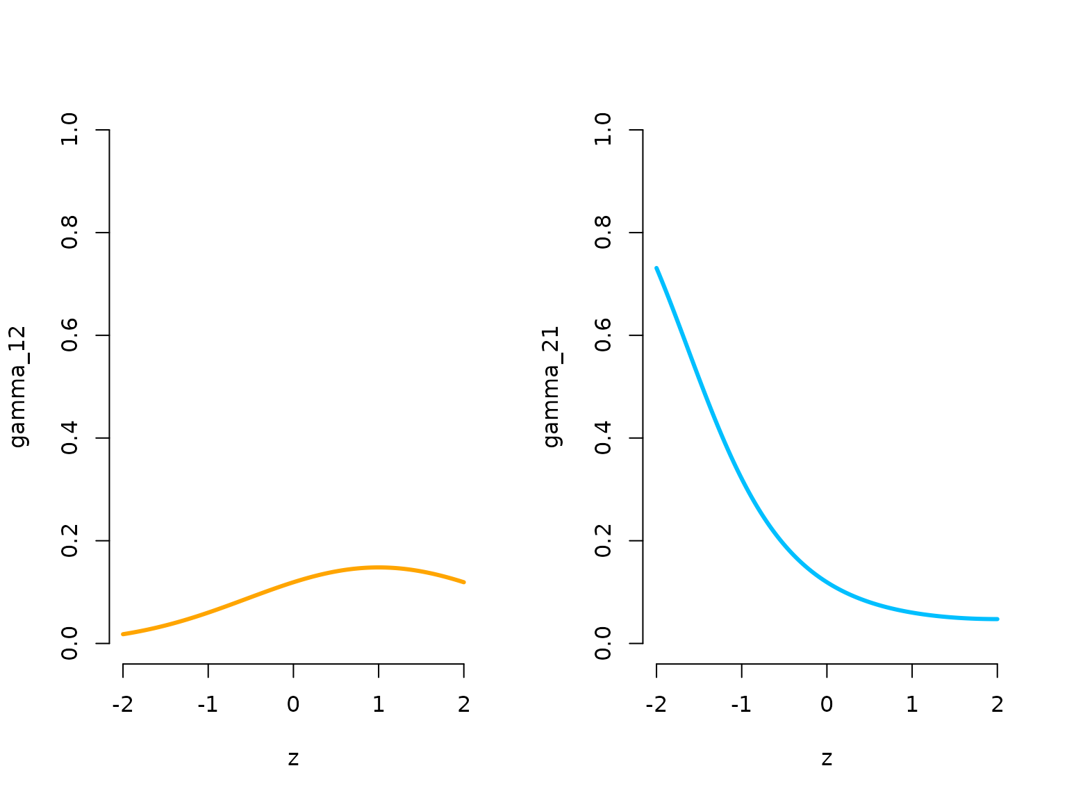
par(oldpar)Let’s now simulate synthetic data from the above specified model.
s = rep(NA, n)
s[1] = sample(1:2, 1, prob = delta) # sampling first state from initial distr.
for(t in 2:n){
  # sampling next state conditional on previous one with tpm at that time point
  s[t] = sample(1:2, 1, prob = Gamma[s[t-1],,t-1])
}
# sampling observations conditional on the states
x = rnorm(n, mu[s], sigma[s])

plot(x[1:200], bty = "n", pch = 20, ylab = "x",
     col = c(color[1], color[2])[s[1:200]])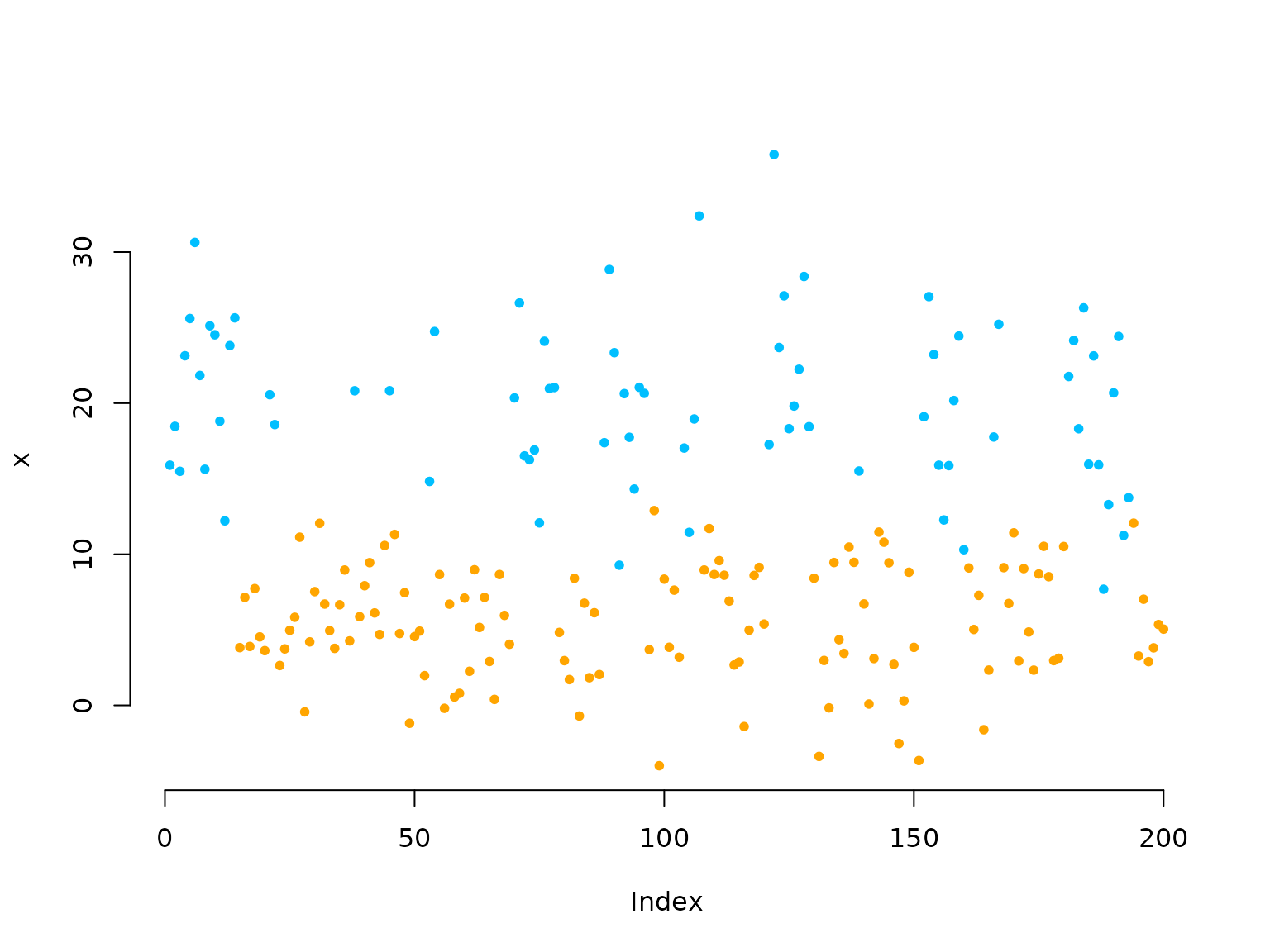
We now model the transition probabilities parametrically, where we have a parameter for the intercept, the linear effect and the quadratic effect for each off-diagonal element of the t.p.m.
Writing the negative log-likelihood function
Here we specify the likelihood function and pretend we know the polynomial degree of the effect of z on the transition probabilities.
nll = function(par, x, Z){
  beta = matrix(par[1:6], nrow = 2) # matrix of coefficients
  Gamma = tpm_g(Z[-1,], beta) # excluding the first covariate value -> n-1 tpms
  delta = c(1, exp(par[7]))
  delta = delta / sum(delta)
  mu = par[8:9]
  sigma = exp(par[10:11])
  # calculate all state-dependent probabilities
  allprobs = matrix(1, length(x), 2)
  for(j in 1:2) allprobs[,j] = dnorm(x, mu[j], sigma[j])
  # forward algorithm
  -forward_g(delta, Gamma, allprobs)
}
Fitting an HMM to the data
par = c(beta = c(-2, -2, rep(0,4)), # initialising with homogeneous tpm
        logitdelta = 0, # starting value for initial distribution
        mu = c(4, 14), # initial state-dependent means
        sigma = c(log(3),log(5))) # initial state-dependents sds
system.time(
  mod <- nlm(nll, par, x = x, Z = Z)

)
#>    user  system elapsed
#>   0.802   0.011   0.813
Really fast!
Visualising results
Again, we use tpm_g() and stationary() to
transform the parameters.
# transform parameters to working
beta_hat = matrix(mod$estimate[1:6], nrow = 2)
Gamma_hat = tpm_g(Z = Z[-1,], beta_hat)
delta_hat = c(1, exp(mod$estimate[7]))
delta_hat = delta_hat / sum(delta_hat)
mu_hat = mod$estimate[8:9]
sigma_hat = exp(mod$estimate[10:11])

# we calculate the average state distribution overall all covariate values
zseq = seq(-2, 2, by = 0.01)
Gamma_seq = tpm_g(Z = cbind(zseq, zseq^2), beta_hat)
Prob = matrix(nrow = length(zseq), ncol = 2)
for(i in 1:length(zseq)){ Prob[i,] = stationary(Gamma_seq[,,i]) }
prob = apply(Prob, 2, mean)

hist(x, prob = TRUE, bor = "white", breaks = 20, main = "")
curve(prob[1]*dnorm(x, mu_hat[1], sigma_hat[1]), add = TRUE, lwd = 3,
      col = color[1], n=500)
curve(prob[2]*dnorm(x, mu_hat[2], sigma_hat[2]), add = TRUE, lwd = 3,
      col = color[2], n=500)
curve(prob[1]*dnorm(x, mu_hat[1], sigma_hat[1])+
        prob[2]*dnorm(x, mu[2], sigma_hat[2]),
      add = TRUE, lwd = 3, lty = "dashed", n = 500)
legend("topright", col = c(color[1], color[2], "black"), lwd = 3, bty = "n",
       lty = c(1,1,2), legend = c("state 1", "state 2", "marginal"))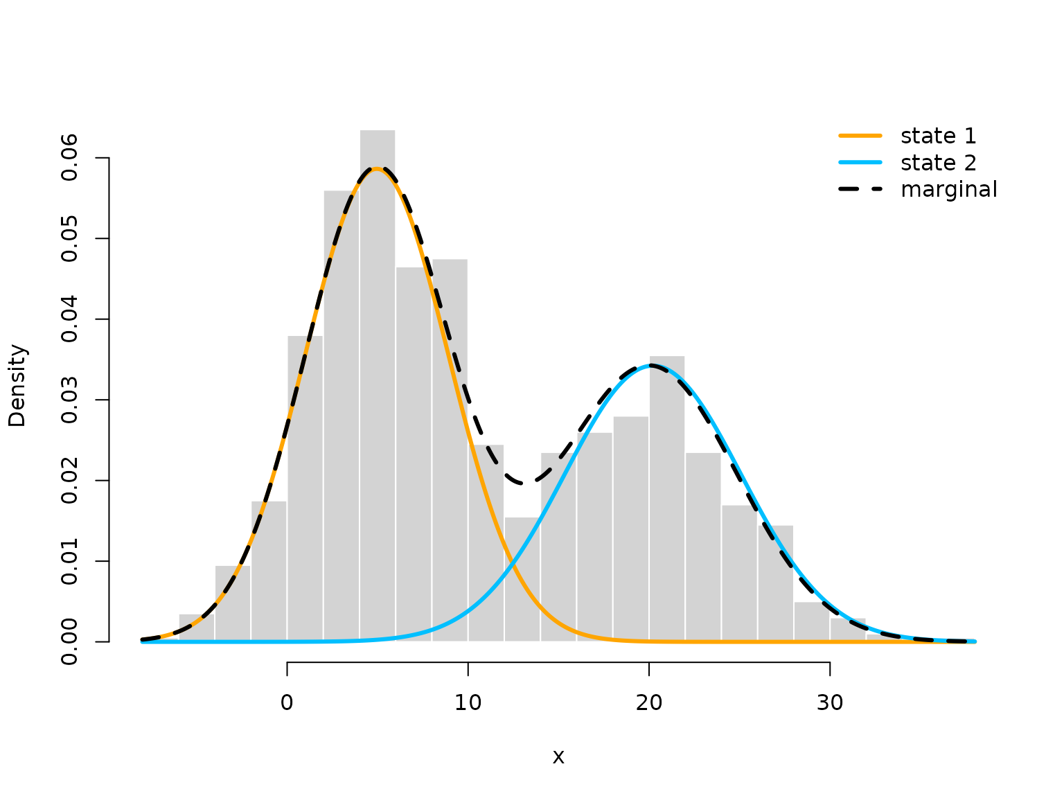
oldpar = par(mfrow = c(1,2))
plot(zseq, Gamma_seq[1,2,], type = "l", lwd = 3, bty = "n", ylim = c(0,1),
     xlab = "z", ylab = "gamma_12_hat", col = color[1])
plot(zseq, Gamma_seq[2,1,], type = "l", lwd = 3, bty = "n", ylim = c(0,1),
     xlab = "z", ylab = "gamma_21_hat", col = color[2])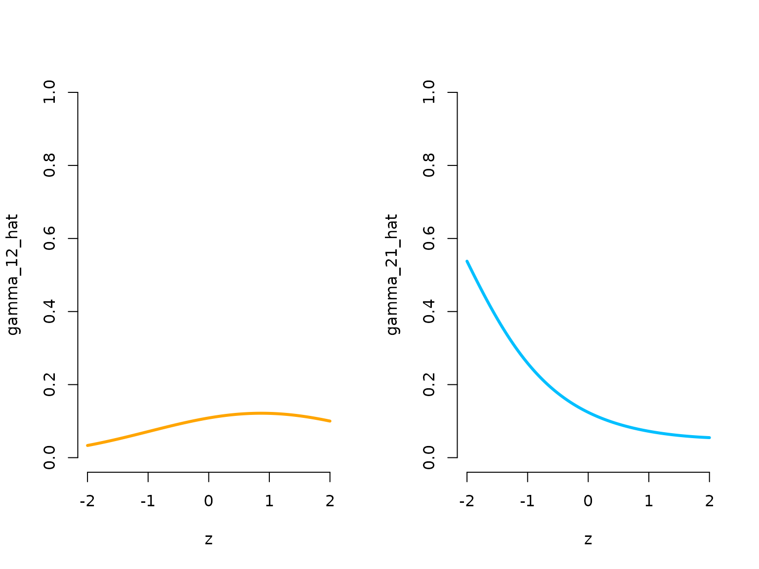
par(mfrow = c(1,1))
plot(zseq, Prob[,1], type = "l", lwd = 3, bty = "n", ylim = c(0,1), xlab = "z",
     ylab = "Pr(state 1)", col = color[1])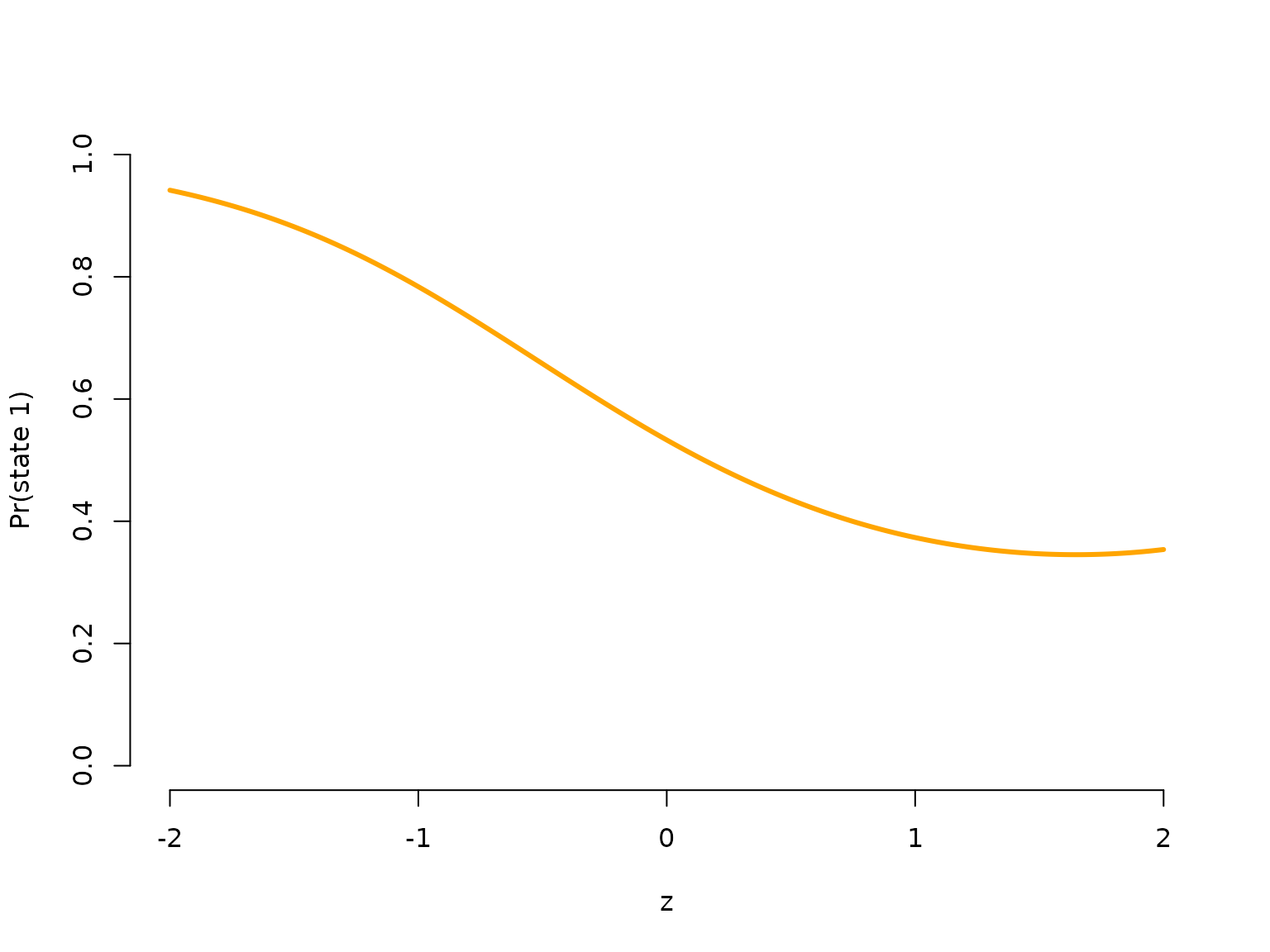
par(oldpar)Covariate effects in the state-dependent process
We now look at a setting where covariates influence the mean of the state-dependent distribution, while the state switching is controlled by a homogeneous Markov chain. This is often called Markov-switching regression. Assuming the observation process to be conditionally normally distributed, this means
X_t \mid S_t = j \sim N(\beta_j^{'} z_t, \: \sigma_j^2), \quad j = 1, \dots, N.
Simulation example
First we specify parameters for the simulation. The important change
here is that beta now contains the regression coefficients
for the state-dependent regressions.
sigma = c(1, 1) # state-dependent standard deviations (homoscedasticity)

# parameter matrix
# each row contains parameter vector for the corresponding state
beta = matrix(c(8, 10,             # intercepts
                -2, 1, 0.5, -0.5), # slopes
              nrow = 2)
n = 1000 # number of observations
set.seed(123)
z = rnorm(n)
Z = cbind(z, z^2) # quadratic effect of z

Gamma = matrix(c(0.9, 0.1, 0.05, 0.95),
               nrow = 2, byrow = TRUE) # homogeneous t.p.m.
delta = stationary(Gamma) # stationary Markov chain
Simulation
In the simulation code, the state-dependent mean now is not fixed
anymore, but changes according to the covariate values in
Z.
s = x = rep(NA, n)
s[1] = sample(1:2, 1, prob = delta)
x[1] = rnorm(1, beta[s[1],]%*%c(1, Z[1,]), # state-dependent regression
                    sigma[s[1]])
for(t in 2:n){
  s[t] = sample(1:2, 1, prob = Gamma[s[t-1],])
  x[t] = rnorm(1, beta[s[t],]%*%c(1, Z[t,]), # state-dependent regression
                      sigma[s[t]])
}

oldpar = par(mfrow = c(1,2))
plot(x[1:400], bty = "n", pch = 20, ylab = "x",
     col = c(color[1], color[2])[s[1:400]])

plot(z[which(s==1)], x[which(s==1)], pch = 16, col = color[1], bty = "n",
     ylim = c(0,15), xlab = "z", ylab = "x")
points(z[which(s==2)], x[which(s==2)], pch = 16, col = color[2])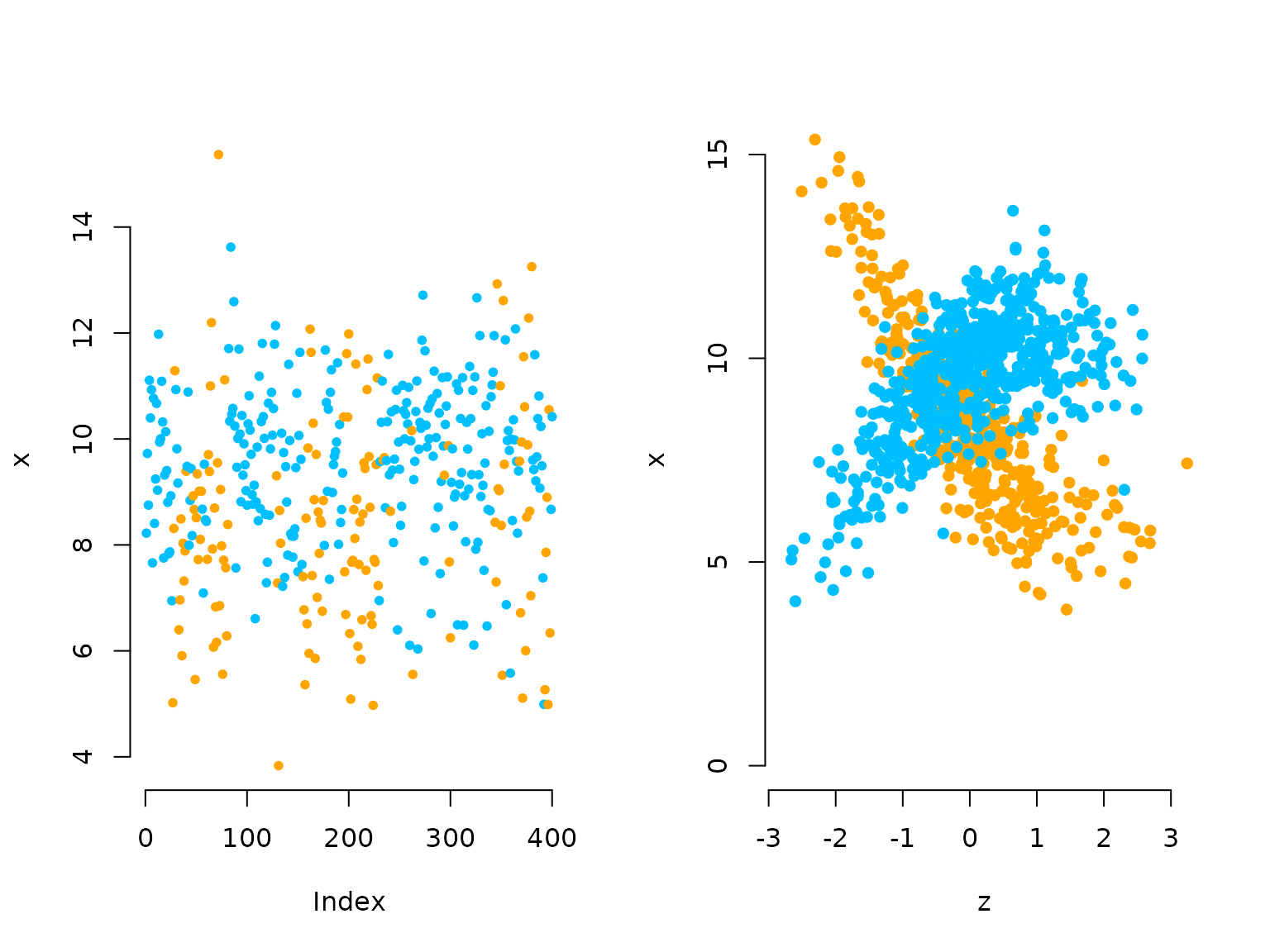
par(oldpar)Writing the negative log-likelihood function
In the likelihood function, we also add the state-dependent
regression in the loop calculating the state-dependent probabilities.
The code cbind(1,Z) %*% beta[j,] computes the linear
predictor for the j-th state.
nllMSR = function(par, x, Z){
  Gamma = tpm(par[1:2]) # homogeneous tpm
  delta = stationary(Gamma) # stationary Markov chain
  beta = matrix(par[2 + 1:(2 + 2*2)], nrow = 2) # parameter matrix
  sigma = exp(par[2 + 2 + 2*2 + 1:2])
  # calculate all state-dependent probabilities
  allprobs = matrix(1, length(x), 2)
  # state-dependent regression
  for(j in 1:2) allprobs[,j] = dnorm(x, cbind(1,Z) %*% beta[j,], sigma[j])
  # forward algorithm
  -forward(delta, Gamma, allprobs)
}Visualising results
To visualise the results, be transform the parameters to working parameters and add the two estimated state-specific regressions to the scatter plot.
Gamma_hat_reg = tpm(mod_reg$estimate[1:2]) # calculating all tpms
delta_hat_reg = stationary(Gamma_hat_reg)
beta_hat_reg = matrix(mod_reg$estimate[2+1:(2*2+2)], nrow = 2)
sigma_hat_reg = exp(mod_reg$estimate[2+2*2+2 +1:2])

# we have some label switching
plot(z, x, pch = 16, bty = "n", xlab = "z", ylab = "x", col = color[s])
points(z, x, pch = 20)
curve(beta_hat_reg[1,1] + beta_hat_reg[1,2]*x + beta_hat_reg[1,3]*x^2,
      add = TRUE, lwd = 4, col = color[2])
curve(beta_hat_reg[2,1] + beta_hat_reg[2,2]*x + beta_hat_reg[2,3]*x^2,
      add = TRUE, lwd = 4, col = color[1])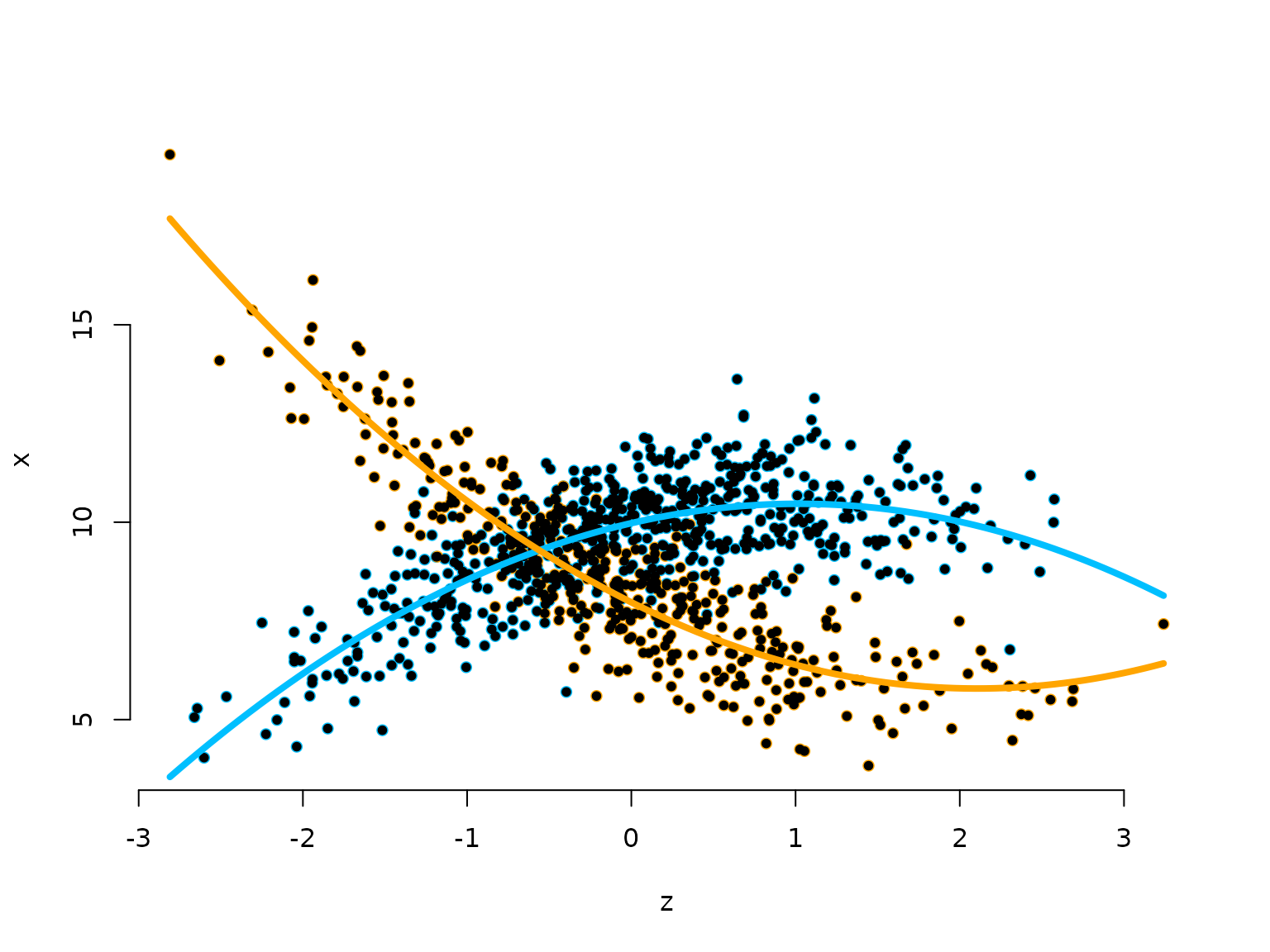
Continue reading with Periodic HMMs, LaMa and RTMB, or Penalised splines.