Worked Examples

library(RTMBdist)

Example 1: Random regression with non-Gaussian data

Our first example is the chicken weight data set, already used in the RTMB Introduction vignette.

We fit the same random regression model, where each chick has its own intercept and slope parameters that are assumed to be normally distributed. However, instead of assuming normal errors, we assume that the observations given the time and chick follow a Box-Cox Cole-Green (BCCG) distribution, which allows for skewness in the data.

data(ChickWeight)

parameters <- list(
  mua=0,          # Mean slope
  log_sda=1,      # log-Std of slopes
  mub=0,          # Mean intercept
  log_sdb=1,      # log-Std of intercepts
  log_sigma=0,    # log-Scale of BCCG distribution
  nu = 0.1,       # Skewness of BCCG distribution
  a=rep(0, 50),   # Random slope by chick
  b=rep(5, 50)    # Random intercept by chick
)

The joint negative log-likelihood function has the same structure as in the RTMB vignette, but with the normal likelihood replaced by the BCCG likelihood, and hence also some necessary parameter transformations.

nll_chick <- function(parms) {
  getAll(ChickWeight, parms, warn=FALSE)
  # Optional (enables extra RTMB features)
  weight <- OBS(weight)
  # Initialise joint negative log likelihood
  nll <- 0
  # Random slopes
  sda <- exp(log_sda); ADREPORT(sda)
  nll <- nll - sum(dnorm(a, mean=mua, sd=sda, log=TRUE))
  # Random intercepts
  sdb <- exp(log_sdb); ADREPORT(sdb)
  nll <- nll - sum(dnorm(b, mean=mub, sd=sdb, log=TRUE))
  # Data
  predWeight <- exp(a[Chick] * Time + b[Chick])
  sigma <- exp(log_sigma); ADREPORT(sigma)
  nll <- nll - sum(dbccg(weight, mu=predWeight, sigma=sigma, nu=nu, log=TRUE))
  # Get predicted weight uncertainties
  ADREPORT(predWeight)
  # Return
  nll
}

The model can then again be fitted by constructing the Laplace-approximated marginal log-likelihood function and optimising this using any standard numerical optimiser.

obj_chick <- MakeADFun(nll_chick, parameters, random=c("a", "b"), silent = TRUE)
opt_chick <- nlminb(obj_chick$par, obj_chick$fn, obj_chick$gr)

We can use RTMB’s automatic simulation capabilities to simulate from the fitted model and run a check whether the Laplace approximation is adequate. All of this is done by a simple call to checkConsistency().

set.seed(1)
checkConsistency(obj_chick)
#> Parameters used for simulation:
#>         mua     log_sda         mub     log_sdb   log_sigma          nu 
#>  0.07799513 -3.86869405  3.80355961 -2.65747574 -2.32420504  3.44873713 
#> 
#> Test correct simulation (p.value):
#> [1] 0.7383633
#> Simulation appears to be correct
#> 
#> Estimated parameter bias:
#>           mua       log_sda           mub       log_sdb     log_sigma 
#> -0.0001346800  0.0064958230 -0.0001147128 -0.0147141495  0.0042912804 
#>            nu 
#> -0.0836398603

Lastly, we can also automatically calculate quantile residuals via probability integral transform using oneStepPredict().

osa_chick <- oneStepPredict(obj_chick, discrete=FALSE, trace=FALSE)
qqnorm(osa_chick$res); abline(0,1)

We see that this model is still not a great fit but a bit better than the Gaussian model.

Example 2: Non-standard random GLM for count data

Our second example is the InsectSprays data set. We will fit a GLMM where the counts are assumed to follow a generalised Poisson distribution, allowing for overdispersion (compared to the standard Poisson distribution). In the model, we simple include a random effect for each spray type, to account for the fact that some sprays are more effective than others.

data(InsectSprays)

# Creating the model matrix
X <- model.matrix(~ spray - 1, data = InsectSprays)

par <- list(
  beta0 = log(mean(InsectSprays$count)),
  beta = rep(0, length(levels(InsectSprays$spray))),
  log_phi = log(1),
  log_sigma = log(1)
)
dat <- list(
  count = InsectSprays$count,
  spray = InsectSprays$spray,
  X = X
)

nll_insect <- function(par) {
  getAll(par, dat, warn=FALSE)
  count <- OBS(count)
  # Random effect likelihood
  sigma <- exp(log_sigma); ADREPORT(sigma)
  nll <- - sum(dnorm(beta, 0, sigma, log = TRUE))
  # Data likelihood
  lambda <- exp(beta0 + as.numeric(X %*% beta)); ADREPORT(lambda)
  phi <- exp(log_phi); ADREPORT(phi)
  nll <- nll -sum(dgenpois(count, lambda, phi, log = TRUE))
  nll
}

obj_insect <- MakeADFun(nll_insect, par, random = "beta", silent = TRUE)
opt_insect <- nlminb(obj_insect$par, obj_insect$fn, obj_insect$gr)

# Checking if the Laplace approximation is adequate
checkConsistency(obj_insect)
#> Parameters used for simulation:
#>      beta0    log_phi  log_sigma 
#>  1.9751913 -3.8913794 -0.2221668 
#> 
#> Test correct simulation (p.value):
#> [1] 0.605786
#> Simulation appears to be correct
#> 
#> Estimated parameter bias:
#>       beta0     log_phi   log_sigma 
#> -0.01672544  0.03395053 -0.00437216
# Check okay

# Calculating quantile residuals
osa_insect <- oneStepPredict(obj_insect, method = "oneStepGeneric", 
                             discrete=TRUE, trace=FALSE)
qqnorm(osa_insect$res); abline(0,1)

Example 3: Distributional regression with penalised splines

Our third example covers the dutch boys BMI data set, part of the gamlss.data package. We will fit a distributional regression model where the location, scale, and skewness parameters of the Box-Cox power exponential (BCPE) distribution are modelled as smooth functions of age using penalised splines. The kurtosis parameter will be kept constant.

We start by loading packages that are needed.

library(gamlss.data)   # Data
library(LaMa)          # Creating model matrices
library(Matrix)        # Sparse matrices

data(dbbmi)
# Subset (just for speed here)
set.seed(1)
ind <- sample(1:nrow(dbbmi), 2000)
dbbmi <- dbbmi[ind, ]

We use the function make_matrices() from package LaMa to conveniently create design and penalty matrices for the smooth functions. Internally, this just interfaces mgcv. The penalty matrix is converted to a sparse matrix using the Matrix package, to work with RTMB’s dgmrf() function.

k <- 10 # Basis dimension
modmat <- make_matrices(~ s(age, bs="cs"), data = dbbmi)
X <- modmat$Z                              # Design matrix
S <- Matrix(modmat$S[[1]], sparse = TRUE)  # Sparse penalty matrix

The joint negative log-likelihood function computes covariate dependent location, scale, and skewness parameters using the design matrix and regression coefficients. The regression coefficients are treated as random effects with a multivariate normal distribution with zero mean and a precision matrix that is a scaled version of the penalty matrix, which is achieved by calling dgmrf() for each of them. The scaling/ smoothing parameters are estimated by restricted maximum likelihood (REML), which is achieved by treating them as fixed effects and integrating out the regression coefficients and other fixed effects using the Laplace approximation.

nll_dbbmi <- function(par) {
  getAll(par, dat, warn=FALSE)
  bmi <- OBS(bmi)
  # Calculating response parameters
  mu <- exp(X %*% c(beta0_mu, beta_age_mu)); ADREPORT(mu) # Location
  sigma <- exp(X %*% c(beta0_sigma, beta_age_sigma)); ADREPORT(sigma) # Scale
  nu <- X %*% c(beta0_nu, beta_age_nu); ADREPORT(nu) # Skewness
  tau <- exp(log_tau); ADREPORT(tau) # Kurtosis
  # Data likelihood: Box-Cox power exponential distribution
  nll <- - sum(dbcpe(bmi, mu, sigma, nu, tau, log=TRUE))
  # Penalised splines as random effects: log likelihood / penalty
  lambda <- exp(log_lambda); REPORT(lambda)
  nll <- nll - dgmrf(beta_age_mu, 0, lambda[1] * S, log=TRUE)
  nll <- nll - dgmrf(beta_age_sigma, 0, lambda[2] * S, log=TRUE)
  nll <- nll - dgmrf(beta_age_nu, 0, lambda[3] * S, log=TRUE)
  nll
}

par <- list(
  beta0_mu = log(18), beta0_sigma = log(0.15),
  beta0_nu = -1, beta_age_mu = rep(0, k-1),
  beta_age_sigma = rep(0, k-1), beta_age_nu = rep(0, k-1),
  log_tau = log(2),
  log_lambda = log(rep(1e4, 3))
)
dat <- list(
  bmi = dbbmi$bmi,
  age = dbbmi$age,
  X = X,
  S = S
)

As we are using REML, we are integrating out all parameters that are not smoothing parameters log_lambda. The model is then fitted by constructing the Laplace-approximated restricted log-likelihood function and optimising this.

# Restricted maximum likelihood (REML) - also integrating out fixed effects
random <- names(par)[names(par) != "log_lambda"]
obj_dbbmi <- MakeADFun(nll_dbbmi, par, random = random, silent = TRUE)
opt_dbbmi <- nlminb(obj_dbbmi$par, obj_dbbmi$fn, obj_dbbmi$gr)

We can have access to all ADREPORT()ed quantities and their standard deviation using sdreport().

sdr <- sdreport(obj_dbbmi, ignore.parm.uncertainty = TRUE)
par <- as.list(sdr, "Est", report = TRUE)
par_sd <- as.list(sdr, "Std", report = TRUE)

This way, we can easily plot the estimated smooth functions with confidence intervals and the conditional distribution of BMI given age.

age <- dbbmi$age
ord <- order(age)

# Plotting estimated effects
oldpar <- par(mfrow = c(1,3))
plot(age[ord], par$mu[ord], type = "l", lwd = 2, bty = "n", xlab = "Age", ylab = "Mu")
polygon(c(age[ord], rev(age[ord])),
        c(par$mu[ord] + 2*par_sd$mu[ord], rev(par$mu[ord] - 2*par_sd$mu[ord])),
        col = "#00000020", border = "NA")
plot(age[ord], par$sigma[ord], type = "l", lwd = 2, bty = "n", xlab = "Age", ylab = "Sigma")
polygon(c(age[ord], rev(age[ord])),
        c(par$sigma[ord] + 2*par_sd$sigma[ord], rev(par$sigma[ord] - 2*par_sd$sigma[ord])),
        col = "#00000020", border = "NA")
plot(age[ord], par$nu[ord], type = "l", lwd = 2, bty = "n", xlab = "Age", ylab = "Nu")
polygon(c(age[ord], rev(age[ord])),
        c(par$nu[ord] + 2*par_sd$nu[ord], rev(par$nu[ord] - 2*par_sd$nu[ord])),
        col = "#00000020", border = "NA")

par(oldpar)

# Plotting conditional distribution
plot(dbbmi$age, dbbmi$bmi, pch = 16, col = "#00000020",
     xlab = "Age", ylab = "BMI", bty = "n")
lines(age[ord], par$mu[ord], lwd = 3, col = "deepskyblue")

# Compute quantiles (point estimates)
par <- lapply(par, as.numeric)
ps <- seq(0, 1, length = 8)
ps[1] <- 0.005 # avoid 0 and 1
ps[length(ps)] <- 0.995 # avoid 0 and 1
for(p in ps) {
  q <- qbcpe(p, par$mu, par$sigma, par$nu, par$tau) # quantiles
  lines(age[ord], q[ord], col = "deepskyblue")
}
legend("topleft", lwd = c(3, 1), col = "deepskyblue", legend = c("Mean", "Quantiles"), bty = "n")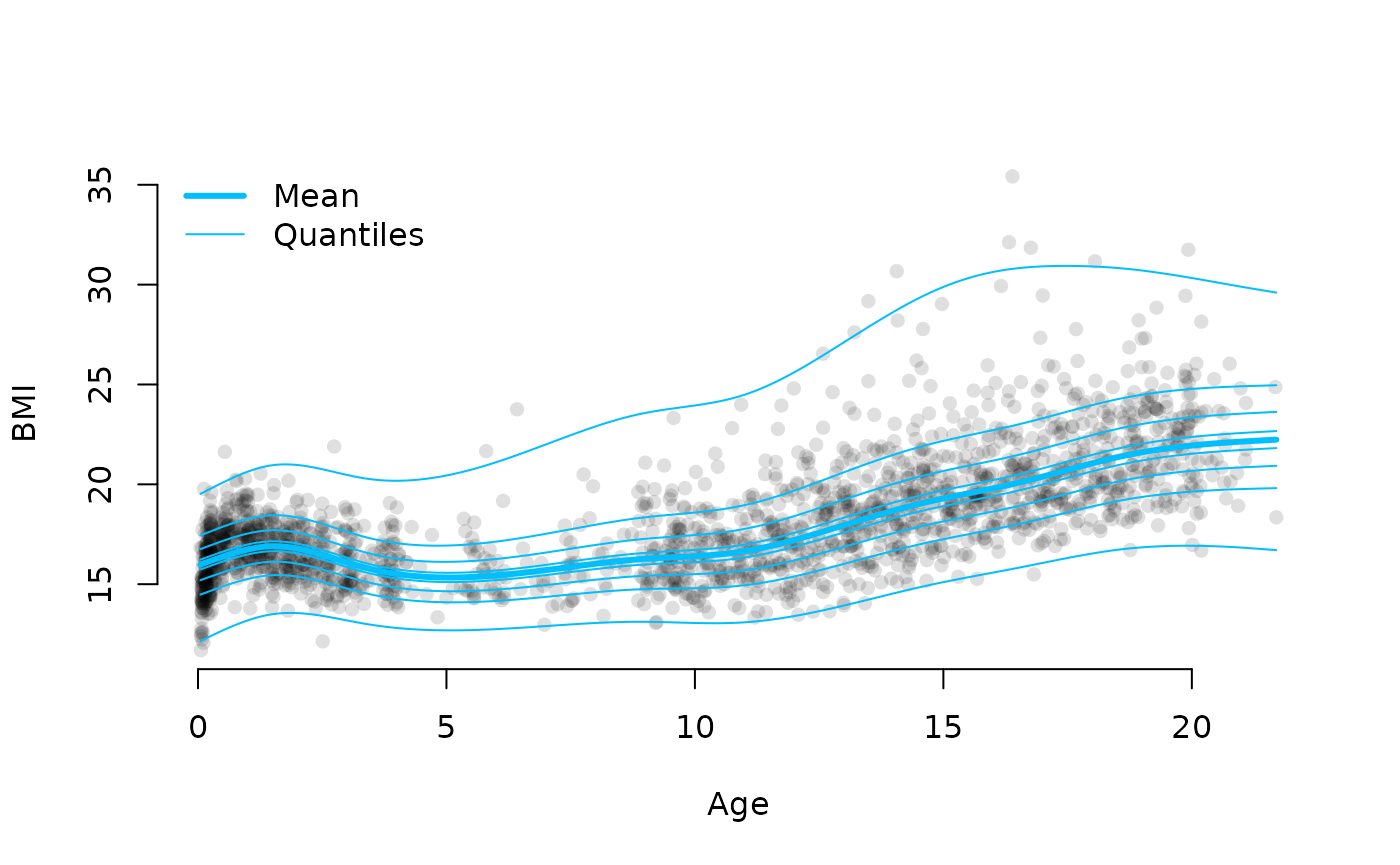

Example 4: Zero inflation

In this example, we look at the aep data set, containing data on the number of inappropriate days spent in the hospital and the length of a stay for patients admitted to a hospital in Barcelona. These data have been analysed by Gange et al. (1996). They fitted a binomial logistic regression model as well as a beta-binomial regression model, concluding that the beta-binomial model produced a better fit. Due to the large number of zeros in the data, we will here also fit a zero-inflated binomial model and compare the results.

library(gamlss.data)
head(aep)
#>   los noinap     loglos sex ward year age y.noinap y.failures
#> 1  15      0  0.4054651   2    2   88   0        0         15
#> 2  42     20  1.4350845   2    1   88  18       20         22
#> 3   8      6 -0.2231436   1    1   88  19        6          2
#> 4   9      6 -0.1053605   1    2   88  23        6          3
#> 5   7      0 -0.3566749   1    2   88   2        0          7
#> 6  10      2  0.0000000   2    2   88  -8        2          8

We start by fitting the 2 binomial models. We only define one likelihood function and fix the zero probability to 0 for the binomial model.

# Defininig the model matrix for the model reported in Gange et al. (1996)
X <- model.matrix(~ age + ward + loglos * year, data = aep)

# (zero-inflated) binomial likelihood
nll_aep <- function(par) {
  getAll(par, dat)
  y <- OBS(y); size <- OBS(size)
  prob <- plogis(X %*% beta); ADREPORT(prob) # linear predictor and link
  zeroprob <- plogis(logit_zeroprob); ADREPORT(zeroprob)
  - sum(dzibinom(y, size, prob, zeroprob, log = TRUE))
}

# Initial parameters
beta_init <- c(-1, rep(0, ncol(X)-1))
names(beta_init) <- colnames(X)
par <- list(beta = beta_init)

dat <- list(
  y = aep$y[,1],
  size = aep$los,
  X = X
)

# Fitting the binomial model (zeroprob fixed at 0)
map <- list(logit_zeroprob = factor(NA)) # fixing at initial value
par$logit_zeroprob <- qlogis(0) # set to zero
obj_aep1 <- MakeADFun(nll_aep, par, silent = TRUE, map = map)
opt_aep1 <- nlminb(obj_aep1$par, obj_aep1$fn, obj_aep1$gr)

# Fitting the zero-inflated binomial model, no parameter restrictions
par$logit_zeroprob <- qlogis(1e-2) # more sensible initial value
obj_aep2 <- MakeADFun(nll_aep, par, silent = TRUE)
opt_aep2 <- nlminb(obj_aep2$par, obj_aep2$fn, obj_aep2$gr)
#> Warning in nlminb(obj_aep2$par, obj_aep2$fn, obj_aep2$gr): NA/NaN function
#> evaluation

# Reporting
sdr_aep1 <- sdreport(obj_aep1)
sdr_aep2 <- sdreport(obj_aep2)

beta1 <- as.list(sdr_aep1, "Est")$beta
beta2 <- as.list(sdr_aep2, "Est")$beta
(zeroprob2 <- as.list(sdr_aep2, "Est", report = TRUE)$zeroprob)
#> [1] 0.4294577

round(rbind(beta1, beta2), 3)
#>       (Intercept)   age  ward2  ward3 loglos year90 loglos:year90
#> beta1      -1.006 0.006 -0.468 -0.615  0.518  0.168        -0.204
#> beta2       0.058 0.009 -0.622 -0.873  0.235 -0.294        -0.087

We find that accounting for the zero-inflation somewhat changes the estimated coefficients. Now we also fit the beta-binomial model. In this model, the shape parameters are modelled as p_i / \theta_i and (1-p_i) / \theta_i, where p_i is the covariate-dependent probability for observation i and \theta_i is a parameter controlling the overdispersion. The parameter \theta_i is modelled as a function of year only, exactly as in Gange et al. (1996).

# Beta-binomial likelihood
nll_aep2 <- function(par) {
  getAll(par, dat)
  y <- OBS(y); size <- OBS(size)
  theta <- plogis(X_theta %*% beta_theta); ADREPORT(theta) # overdispersion parameter
  prob <- plogis(X %*% beta); ADREPORT(prob) # linear predictor and link
  - sum(dbetabinom(y, size, prob / theta, (1-prob) / theta, log = TRUE))
}

# Design matrices
X <- model.matrix(~ ward + loglos + year, data = aep)
X_theta <- model.matrix(~ year, data = aep)

# Initial parameters
beta <- c(-1, rep(0, ncol(X)-1)); names(beta) <- colnames(X)
beta_theta <- c(1, 0); names(beta_theta) <- colnames(X_theta)

par <- list(beta = beta, beta_theta = beta_theta)
dat <- list(
  y = aep$y[,1],
  size = aep$los,
  X = X, 
  X_theta = X_theta
)

obj_aep3 <- MakeADFun(nll_aep2, par, silent = TRUE)
opt_aep3 <- nlminb(obj_aep3$par, obj_aep3$fn, obj_aep3$gr)

sdr_aep3 <- sdreport(obj_aep3)

beta3 <- as.list(sdr_aep3, "Est")$beta

round(beta3, 3)
#> (Intercept)       ward2       ward3      loglos      year90 
#>      -1.126      -0.320      -0.606       0.537       0.295

Example 5: Copulas

For this example, we are modelling the faithful data set. It contains measurements of the waiting time between eruptions and the duration of the eruption for the Old Faithful geyser in Yellowstone National Park, Wyoming, USA. We will fit a mixture of two bivariate distributions, where each component has normal marginal distributions and a Clayton copula to model the dependence between the two variables.

data(faithful)

Specifying the mixture likelihood using dcopula() and cclayton() for the components is straightforward, it’s just imporant to not confuse mixture components and dimensions.

nll_copula <- function(par) {
  getAll(par, faithful)
  REPORT(mu1); REPORT(mu2)
  sigma1 <- exp(log_sigma1); REPORT(sigma1) # marginal sds component 1
  sigma2 <- exp(log_sigma2); REPORT(sigma2) # marginal sds component 2
  theta <- exp(log_theta); REPORT(theta) # dependence parameters
  alpha <- exp(log_alpha); REPORT(alpha) # mixture weights
  # Marginal densities
  # Margin 1: Waiting
  d1 <- cbind(dnorm(waiting, mu1[1], sigma1[1], log=TRUE), # Component 1
              dnorm(waiting, mu2[1], sigma2[1], log=TRUE)) # Component 2
  # Margin 2: Eruptions
  d2 <- cbind(dnorm(eruptions, mu1[2], sigma1[2], log=TRUE), # Component 1
              dnorm(eruptions, mu2[2], sigma2[2], log=TRUE)) # Component 2
  # Marginal CDFs
  # Margin 1: Waiting
  p1 <- cbind(pnorm(waiting, mu1[1], sigma1[1]), # Component 1
              pnorm(waiting, mu2[1], sigma2[1])) # Component 2
  # Margin 2: Eruptions
  p2 <- cbind(pnorm(eruptions, mu1[2], sigma1[2]), # component 1
              pnorm(eruptions, mu2[2], sigma2[2])) # component 2
  
  # Computing mixture likelihood:
  ll1 <- dcopula(d1[,1], d2[,1], p1[,1], p2[,1], cclayton(theta[1]), log=TRUE) # f1(x,y)
  ll2 <- dcopula(d1[,2], d2[,2], p1[,2], p2[,2], cclayton(theta[2]), log=TRUE) # f2(x,y)
  # alpha * f1(x,y) + (1-alpha) * f2(x,y) on log scale for each obervation
  ll <- logspace_add(log_alpha + ll1, log1p(-alpha) + ll2) 
  - sum(ll) # returning negative sum
}

We fit the model as usual, now using reporting to easily extract the estimated parameters on their natural scale:

# Initial parameters
par <- list(
  mu1 = c(55, 2), mu2 = c(80, 4),
  log_sigma1 = log(c(10, 1)), log_sigma2 = log(c(10, 1)),
  log_theta = log(c(0.5, 0.5)),
  log_alpha = log(0.5)
)

obj_copula <- MakeADFun(nll_copula, par, silent = TRUE)
opt_copula <- nlminb(obj_copula$par, obj_copula$fn, obj_copula$gr)

mod_copula <- obj_copula$report()

# Extract transformed parameters
mu1    <- mod_copula$mu1
mu2    <- mod_copula$mu2
sigma1 <- mod_copula$sigma1
sigma2 <- mod_copula$sigma2
theta  <- mod_copula$theta
alpha  <- mod_copula$alpha

We can plot the result:

# Scatterplot
plot(faithful$waiting, faithful$eruptions, pch = 20, bty = "n",
     xlab = "Waiting time", ylab = "Eruption time", col = "#00000070")

# Grid for evaluation
xseq <- seq(min(faithful$waiting), max(faithful$waiting), length.out = 80)
yseq <- seq(min(faithful$eruptions), max(faithful$eruptions), length.out = 80)

# Evaluate component densities on grid
f1 <- outer(xseq, yseq, function(x,y){
  d1c1 <- dnorm(x, mu1[1], sigma1[1])
  d2c1 <- dnorm(y, mu1[2], sigma1[2])
  p1c1 <- pnorm(x, mu1[1], sigma1[1])
  p2c1 <- pnorm(y, mu1[2], sigma1[2])
  dcopula(d1c1, d2c1, p1c1, p2c1, cclayton(theta[1]))
})
f2 <- outer(xseq, yseq, function(x,y){
  d1c2 <- dnorm(x, mu2[1], sigma2[1])
  d2c2 <- dnorm(y, mu2[2], sigma2[2])
  p1c2 <- pnorm(x, mu2[1], sigma2[1])
  p2c2 <- pnorm(y, mu2[2], sigma2[2])
  dcopula(d1c2, d2c2, p1c2, p2c2, cclayton(theta[2]))
})

# Add contours
contour(xseq, yseq, alpha * f1, add = TRUE, nlevels = 8,
        drawlabels = FALSE, col = "orange", lwd = 2)
contour(xseq, yseq, (1-alpha) * f2, add = TRUE, nlevels = 8,
        drawlabels = FALSE, col = "deepskyblue", lwd = 2)

Example 6: Multivariate stochastic volatility

This example reproduces one of the TMB examples. It fits a multivariate stochastic volatility model to financial returns data. In the example given here, the response distribution is a multivariate Gaussian, with the marginal variance for each of the three time series being time-varying and modelled based on a latent volatility process. We generalise the example to a multivariate t distribution, which typically results in a better fit to financial returns data, due to the heavier tails.

We get the data from

source("https://raw.githubusercontent.com/kaskr/RTMB/master/tmb_examples/sdv_multi_data.R")

The code below is basically the same as in the original example, but uses a multivariate t distribution (dmvt()) in the data likelihood. Note that the Cov matrix is now not actually the covariance matrix anymore, but only proportional to it.

# Multivatiate SV model from Table 5 of Skaug and Yu "A flexible and automated likelihood based 
# framework for inference in stochastic volatility models." Computational Statistics & Data Analysis 76 (2014): 642-654.

## Parameter initial guess
par <- list(
  logit_phi  = qlogis(rep(0.97,p)),       # See eqn (12) in Skaug and Yu (2014)
  log_sigma  = log(rep(0.2,p)),           #       ---------||---------
  mu_y       = rep(-0.5,p),               #       ---------||---------
  off_diag_x = rep(0,p),                  #       ---------||---------
  h          = matrix(0,nrow=n,ncol=p),   #       ---------||---------
  log_df     = log(20)                    # this allows for heavier tails
)

# Negative joint likelihood (nll) of data and parameters
nll_svt <- function(par) {
  getAll(par)
  # Optionally mark the observation object
  y <- OBS(y)
  
  # Parameters on natural scale
  sigma <- exp(log_sigma)
  phi <- plogis(logit_phi)
  sigma_init <- sigma / sqrt(1-phi^2)
  df <- exp(log_df)
  
  nll <- 0  # Start collecting contributions
  
  # Prior on state variable (h)
  nll <- nll - sum(dnorm(h[1,], 0, sigma_init, log=TRUE))   # Start in stationary distribution
  for(j in 1:p) {
    nll <- nll - sum(dnorm(h[-1,j], phi[j]*h[-n,j], sigma[j], log=TRUE))  # AR(1) process for each dimension
  }
  
  # Parameterizes correlation matrix of X in terms of Cholesky factor
  L <- diag(p)
  L[lower.tri(L)] <- off_diag_x   
  row_norms <- apply(L, 1, function(row) sqrt(sum(row^2)))
  L <- L / row_norms
  R <- L %*% t(L)  # Correlation matrix of X (guarantied positive definite)
  
  # Likelihood of data y given h
  for(i in 1:n){
    sigma_y <- exp(0.5 * (mu_y + h[i,])) # variance depending on state
    Cov <- diag(sigma_y) %*% R %*% diag(sigma_y)
    nll <- nll - sum(dmvt(y[i,], 0, Cov, df, log = TRUE))
  }
  nll
}

obj_svt <- MakeADFun(nll_svt, par, random="h", silent = TRUE)
system.time(
  opt_svt <- nlminb(obj_svt$par, obj_svt$fn, obj_svt$gr)
)
#>    user  system elapsed 
#>  16.800  10.822  14.684
rep <- sdreport(obj_svt)
rep
#> sdreport(.) result
#>              Estimate Std. Error
#> logit_phi   3.6269542 0.49413568
#> logit_phi   3.1290137 0.38240912
#> logit_phi   4.7269255 0.80777552
#> log_sigma  -1.9420595 0.21824559
#> log_sigma  -2.0048373 0.17178092
#> log_sigma  -2.4015626 0.34312782
#> mu_y       -1.1388822 0.18663075
#> mu_y       -1.0938327 0.11876150
#> mu_y       -1.5630285 0.31299779
#> off_diag_x -1.3641053 0.06465394
#> off_diag_x -1.1315426 0.06265752
#> off_diag_x  0.7446955 0.04688460
#> log_df      1.9632807 0.13715707
#> Maximum gradient component: 0.000929874